Figures & data
Figure 1 Experimental setup and representative solid specimen.
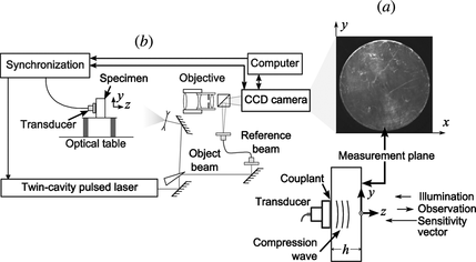
Figure 2 Sketch of the 3-D Fourier transform method. Only three maps are shown for simplicity. An actual sequence would contain a power-of-two number of maps N, typically N = 64 or N = 128. (a) Sequence ΔΦ of optical phase-change maps that contain the spatial and temporal evolution of the out-of-plane displacement at the measurement surface. (b) Complex-valued 3-D spectrum obtained by a 3-D Fourier transform of the sequence in (a); only the modulus is shown. (c) Bandpass filtered 3-D spectrum; only the modulus is shown. (d) Sequence of complex-valued maps that contain the acoustic amplitude and phase at the measurement surface.
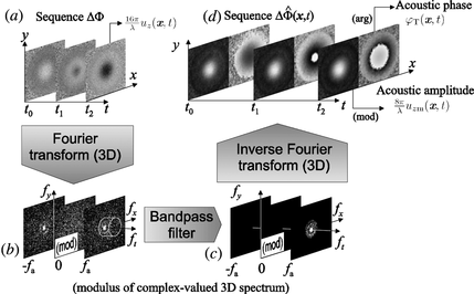
Figure 3 Geometry of the numerical reconstruction process.
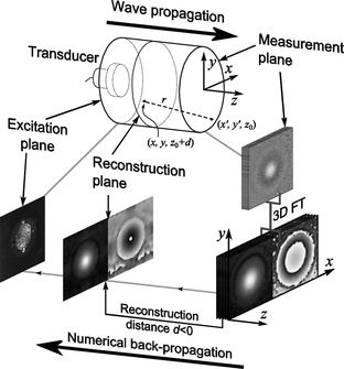
Table 1. Experimental values of the dimensions, acoustic wavelength and phase velocity for f a = (1.00 ± 0.01) MHz in each specimen. The number of cycles per excitation burst used in the experiments is also displayed. All expanded uncertainties are determined with a coverage factor k = 2
Figure 4 Maps of (a) the acoustic amplitude and (b) the acoustic phase reconstructed at 50 mm below the surface of specimen S1. (c) Stack of the transversal profiles of acoustic amplitude at y = 45.00 mm—indicated by the arrows in (a)— obtained for all the reconstruction distances. (d) Longitudinal profile of the acoustic amplitude at position (x,y) = (45.00, 45.00) mm. This line is the intersection of the acoustic amplitude surface shown in (c) with a plane perpendicular to the x-axis at x = 45.00 mm. (e) Top-view of the data set of acoustic amplitude shown in subfigure (c). If the acoustic phase is plotted instead of the acoustic amplitude, the result shown in (f) is obtained.
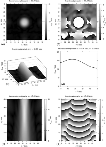
Figure 5 The results obtained in three experiments of simulated defective coupling are shown in columns (ii) to (iv). The maps in columns (ii) and (iii) were obtained with specimen S1. The corresponding results for the same specimen and homogeneous coupling are shown in column (i) for comparison. Results in column (iv) were obtained with the thinnest specimen, S3. Row (a) shows the measured optical phase-change maps, located at position n = 13 in their respective sequences. Row (b) contains the corresponding acoustic amplitude maps (i.e., mod()). Rows (c) to (f) show the acoustic amplitude reconstructed from
within the specimen at the distances indicated. Row (g) is a white-light image of the transducer after the specimens were carefully removed. The field of view is 75.6 mm × 75.6 mm in column (iv), and 90.0 mm × 90.0 mm in the other cases.
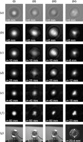
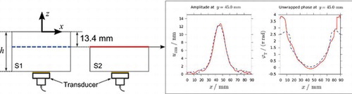
Figure 6 Dashed lines: transversal profiles of acoustic amplitude and unwrapped phase measured at the surface of S1 and then backpropagated within the specimen. Solid lines: transversal profiles of acoustic amplitude and unwrapped phase measured at the surface of the thinner specimen S2. The reconstruction distance was set to −13.4 mm, the difference between the average thicknesses of the samples. Therefore, the reconstructed and measured fields are located at the same distance relative to the transducer.