Acousto-optic coupling in 1-D phoxonic potential well nanobeam cavity using slow modes

Figures & data

Figure 1. (a) The top view and side view of the fishbone unit cell with geometric parameters. The (b) phononic band structure and (c) photonic band structure are shown by blue circles with the SS mode and SL mode indicated by red circles and red arrow respectively in the corresponding figure. (d) The displacement field distribution of the SS mode and (e) the electric field in x-component of the SL mode are depicted below the band structures.

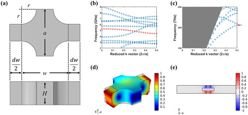
Figure 2. The resonance frequency of the SS mode and the SL mode varying with (a) the wing length dw and (b) the lattice constant a’.

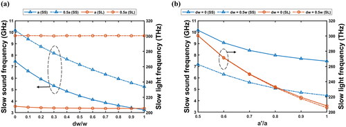
Figure 3. (a) The full sketch of the fishbone nanobeam cavity with parameter denotations. (b) The PnPW line shape of the Type α and β structures. (c) The displacement field of the SS mode at 5.744 GHz and (d) the Ex field distribution of the SL mode calculated by the eigenvalue solver in Type α structure.

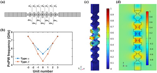
Table 1. Geometry parameter ratio of all the six types of fishbone structures.

	Type α		Type β		Type A		Type B		Type C		Type D
Unit number	a‘/a	dw/w	a‘/a	dw/w	a‘/a	dw/w	a‘/a	dw/w	a‘/a	dw/w	a‘/a	dw/w
0	1	0.3	1	0.5	0.9	0.3	0.9	0.5	1.1	0.3	1.1	0.5
−1/1	1	0.2	1	0.3	0.8	0.2	0.8	0.3	0.9	0.2	0.9	0.3
−2/2	1	0.1	1	0.1	0.7	0.1	0.7	0.1	0.7	0.1	0.7	0.1
−3/3	1	0	1	0	0.6	0	0.6	0	0.6	0	0.6	0

Figure 4. (a) The displacement field of the SS mode at 5.137 GHz and (b) the Ex field distribution of the SL mode calculated by the eigenvalue solver in Type β structure.

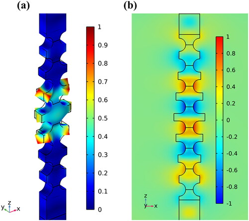
Figure 5. (a) The PnPW line shape and (b) The PtPW line shape of the Type A to D structures. The inset show the tiny difference between Type A, B and Type C, D.

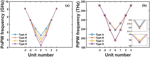
Figure 6. (a) The displacement field of the SS mode at 6.283 GHz and (b) the Ex field distribution of the SL mode calculated by the eigenvalue solver in Type A structure. (c) The displacement field of the SS mode at 5.717 GHz and (d) the Ex field distribution of the SL mode calculated by the eigenvalue solver in Type B structure.

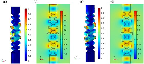
Table 2. Resonant frequencies of the SS modes and SL modes and the coupling rates of the six types fishbone structures.

Type	fSS (GHz)	fSL (THz)	gPE (MHz)	gMB (MHz)	g (MHz)
α	5.7436	203.54	−0.0057	−0.1039	−0.1096
β	5.1373	204.30	0.0141	−0.5774	−0.5633
A	6.2833	216.68	0.0104	−0.8789	−0.8685
B	5.7173	216.92	0.0132	−0.9118	−0.8986
C	5.7717	201.76	0.0764	−1.2850	−1.2086
		214.76	−0.0239	−1.2050	−1.2289
D	5.2173	201.80	0.0406	−0.5917	−0.5511
		214.88	−0.0083	−0.6713	−0.6796

Figure 7. (a) The displacement field of the SS mode in Type C structure at 5.772 GHz. The E_x field distribution of (b) the first-order SL mode and (c) the second-order SL mode calculated by the eigenvalue solver in Type C structure are shown. The dashed line in (b) represents the symmetry axis of the cavity, and the arrows in (c) indicate the center of the −1 and 1 unit cells.

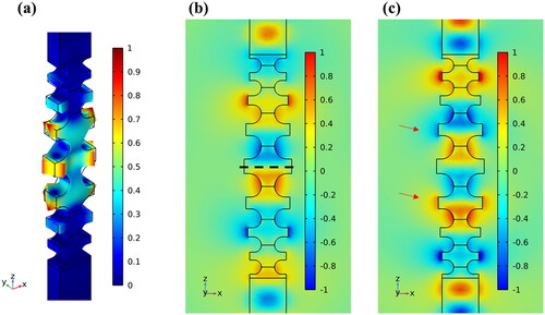
Figure 8. (a) The displacement field of the SS mode in Type D structure at 5.2173 GHz. The E_x field distribution of (b) the first-order SL mode and (c) the second-order SL mode calculated by the eigenvalue solver in Type D structure are shown. The dashed line in (b) represents the symmetry axis of the cavity.

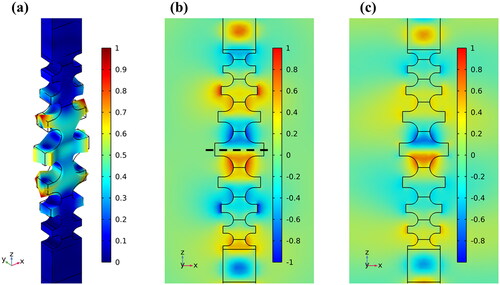
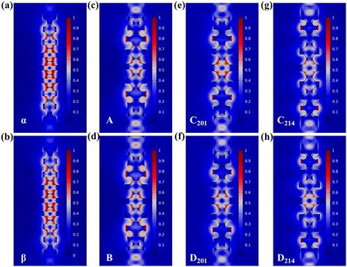
Figure 9. The EM energy of the SL modes in all the six types of fishbone structures. The field distributions represent the corresponding structure that denoted at the left bottom corner of each figure, which are (a) Type α, (b) Type β, (c) Type A, (d) Type B, (e) Type C in 201 THz, (f) Type D in 201 THz, (g) Type C in 214 THz, and (h) Type D in 214 THz.