Figures & data
Figure 1. System configuration and the schematic of the handheld microinjection system for precise subretinal injection.
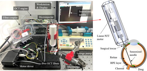
Figure 2. (a) Schematic diagrams of beam profiles exiting from the SMF and GIF-SMF along the z-axis. (b) Image of fusion splicer and fiber polisher. (c) Fiber fusing procedure. (d) Fiber polishing with a desired polishing angle, α. (e) SNR roll-of results from a mirror at 90° and an anodized aluminum plate at 45°.
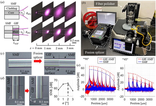
Figure 3. (a) and (b) the microscopic images of the fabricated sensorized needle. (c) Reference coordinates and system parameters of the needle.
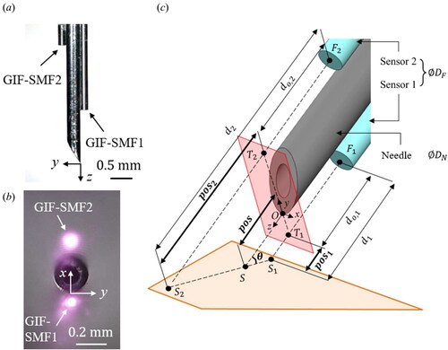
Figure 4. (a) The schematic diagram of the calibration setup. (b) Representative A-lines obtained by the implemented sensorized needle. (c) The calibrated angle measurement results from 40 ° and 140 °. (d) Comparison of the position measurement results at 45 °.
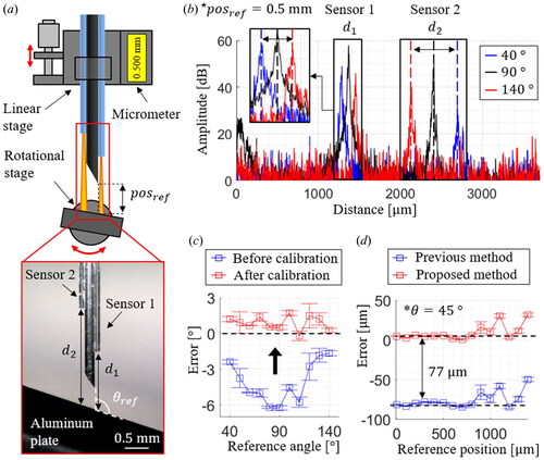
Figure 5. The schematic of the proposed control algorithm. (a) Two operation modes of the handheld microinjector: distance-locking and injection. (b) The block diagram of the position regulation feedback loop using the proposed time delay controller.
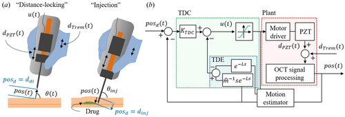
Figure 6. The control gain optimization of (a) P, (b) PID, and (c) TDC. (d) The comparison of the step responses and (e) the motor inputs by the conventional methods and the proposed TDC method with the optimized control gain.
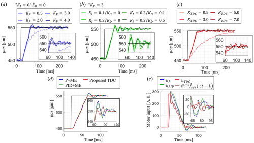
Figure 7. (a) Schematic diagram of the experiment on the recorded tremor. (b) Representative tracking results on the simulated hand tremor at 45°.
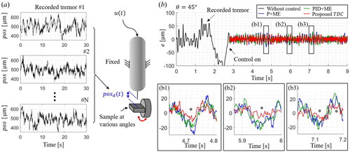
Figure 8. (a) RMSE control results of each control method at several angles. (b) Comparison of position regulation results by each control method.
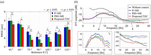
Figure 9. Injection performances on the eyeball phantom made of 2 % agarose-gel. (a) Schematic of the injection experiment with three injection points at tilted angles of 45 °, 90 °, and 135 °. (b) The representative θ and pos measurement results during the one-cycle injection experiment. (c) The representative microscopic images, OCT images, and pos measurements during the injection at each desired point. (d) Comparison of RMSE results during the injection for each control method.
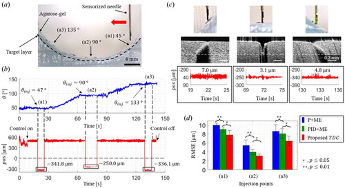
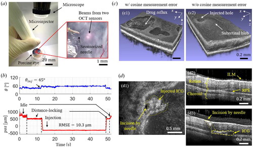
Figure 10. Injection results on an ex-vivo porcine eye. (a) Experimental setup image of the porcine eye injection and the microscopic image of the sensorized needle. (b) Representative θ and pos measurement results during the ex-vivo porcine eye experiment. (c) 3D OCT images of the injected ex-vivo porcine eye (c1) with cosine measurement error and (c2) without cosine measurement error. (d) 2D OCT images: (d1) en-face image of the injected layer and cross-section images of both (d2) non-injected and (d3) injected area.