Prohibition rules for three-node substructures in ordered food webs with cannibalistic species

Figures & data

Figure 1. The 64 ordered three-node substructures without self-links. The index (rank or niche position) of a node increases from bottom to top for each substructure. The horizontal displacement of nodes is only for illustrative purposes. Shaded rectangles mark the substructures that are always prohibited in both the original and the generalised niche model, irrespective of the cannibalistic configuration. The integer index m ∈ [0; 63] is a decimal form of the binary number formed by the off-diagonal elements of the adjacency matrix.

Figure 2. All substructures of Figure 1 have 8 possible configurations describing the presence and absence of self-links. It is illustrated for substructure 15. Shaded rectangles mark the substructures that are prohibited in both the original and the generalised niche model.

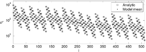
Figure 3. The spectrum of the directed random graph with cannibalistic links. Circles – analytical prediction, dots – numerical results obtained from 40,000 initialisations of the random graph with N = 100, p_↑ = 0.3, p_↓ = 0.4, and p_s = 0.1. The index i is the decimal form of binary number formed by 0s and 1s of the adjacency matrix.

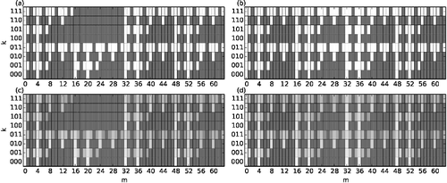
Figure 4. Spectra of three-node substructures in the niche model (a) and (c) and the generalised niche model (b) and (d). (a) and (b) Substructures that appear with nonzero (zero) probability are marked with white (grey) boxes. (c) and (d) Cumulative spectra in logarithmic representation (log(1 + η_km)) of 10,000 initialisations of both niche model variants with N = 100 species and connectance C = 0.1. In the generalised niche model, the factor that reduces the contiguous feeding range of predators is set to c = 0.8. Dark grey corresponds to zero probability, white corresponds to maximal probability.

Figure 5. Cumulative spectrum of empirical food webs in logarithmic representation (log(1 + η_km)). Substructures that are prohibited in both variants of the niche model but present in the empirical data are emphasised. Substructures that are allowed in the niche model or that occur with zero density are marked by dark grey colour, and substructures that are allowed in the generalised niche model but prohibited in the niche model are crossed out with a single line. The only substructure that is not observed in the empirical data-set, (101,45), is emphasised with a white frame. Dark grey corresponds to zero occurrence η_k,m, white corresponds to maximal occurrence η_k,m. All substructures that are allowed in the models are also observed in the empirical data (cf. Figure 6).

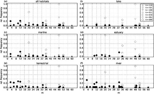
Figure 6. Quantitative spectra of connected three-node substructures in (a) the entire data-set of 63 natural food webs, (b) lake food webs, (c) marine food webs, (d) estuary food webs, (e) terrestrial food webs, and (f) river or stream food webs. Substructures that are prohibited in the niche model and in the generalised niche model are marked with black symbols, substructures that are allowed in the generalised niche model but prohibited in the niche model are marked with grey symbols, and substructures that are allowed in both models are marked with open symbols. Substructures that appear with relative frequency < 0.02 are omitted in this plot. Frequencies are normalised to the occurrence of the most frequent connected substructure, (000,20) in estuary food webs and (000,48) in all other cases.