Modelling runoff reduction through implementation of green and grey roofs in urban catchments using PCSWMM

Figures & data

Figure 1. Green and grey roof in cross-section used in the implementation strategy within the experimental catchment

Figure 2. Location map (the city of Trondheim marked by the yellow star), Risvollan catchment with gauging station (marked by the blue star), the stormwater drainage network, and flat roofs (marked yellow) chosen for green and grey roofs implementation. In total, 45 subcatchments form the whole catchment and 25 subcatchments contain flat roofs (pitched roofs were not considered) which are potential for retrofitting

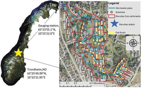
Table 1. The selected monitored and evaluation periods, including date, precipitation depth, precipitation duration, peak precipitation, event duration, runoff depth, and runoff coefficient. The events in bold were considered as warm-period events

Event nr.	Date	Precipitation depth [mm]	Prec. duration [hr]	Peak prec. [mm/hr]	Event duration [hr]	Runoff depth [mm]	Runoff coefficient
C1	16/01/17	50.8	199.0	12	308	65.4	1.29
C2	15/02/17	40	85.9	6	162	11.6	0.29
C3	13/03/17	18.7	63.5	12	75	18.1	0.97
C4	19/04/17	43.3	89.5	12	128	16.0	0.37
C5	21/05/17	15.9	34.5	18	40	2.4	0.15
C6	04/06/17	8.9	15.6	12	25	2.0	0.22
C7	16/06/17	77.5	261.8	18	300	29.2	0.38
C8	10/07/17	46.1	194.6	24	217	12.9	0.28
C9	01/08/17	2.9	2.8	24	7	0.9	0.29
C10	15/08/17	62.7	116.6	36	158	20.8	0.33
C11	29/08/17	3.2	7.1	30	29	3.1	0.98
C12	03/10/17	34.7	128.4	24	139	8.4	0.24
C13	17/10/17	9.4	11.9	18	24	2.8	0.30
C14	27/10/17	84.4	158.2	36	168	35.7	0.42
C15	18/12/17	50.5	121.0	12	135	31.6	0.63
	Min	3	3	6	7	1	0.15
	Max	84	262	36	308	65	1.29
	Mean	37	99	20	128	17	0.48
	Median	40	90	18	135	13	0.33
	Total	549	1490		1915	261	0.48
Event nr.	Date	Precipitation depth [mm]	Prec. duration [hr]	Peak prec. [mm/hr]	Event duration [hr]	Runoff depth [mm]	Runoff coefficient
V1	23/01/18	7.4	85	6	104	0.8	0.11
V2	18/03/18	29.6	96	18	184	12.9	0.43
V3	19/04/18	15.6	51	36	73	10.9	0.70
V4	11/05/18	12.9	12	6	16	1.9	0.15
V5	19/06/18	9.7	3	66	4	0.8	0.09
V6	18/07/18	3.5	2	12	4	0.6	0.16
V7	04/08/18	25.6	35	24	39	5.5	0.21
V8	08/08/18	52.4	57	18	89	20.3	0.39
V9	17/08/18	9.2	1	126	3	0.4	0.05
V10	29/08/18	8.2	4	6	10	1.8	0.22
V11	15/09/18	13.4	68	6	72	2.9	0.22
V12	25/09/18	75.6	137	36	173	38.2	0.50
V13	12/10/18	26	160	12	160	11.1	0.43
V14	16/11/18	10.9	8	24	11	1.4	0.13
V15	24/12/18	82	182	18	186	56.5	0.69
	Min	4	1	6	3	0	0.05
	Max	82	182	126	186	56	0.70
	Mean	25	60	28	75	11	0.30
	Median	13	51	18	72	3	0.22
	Total	382	901		1127	166	0.43

Figure 3. A flowchart of the methodology of the study

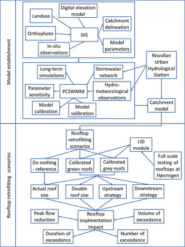
Table 2. Tested rooftops scenarios

Designation	Roof area	Scenario type	Note
A	Actual [1]	Do nothing	Tables 5, 6, A2, and A3
B	Actual [1]	Green roofs	Table 5
C	Actual [1]	Grey roofs	Table 5
D	Double [2]	Green roofs	Table 6
E	Double [2]	Grey roofs	Table 6
F	Actual [1]	Green roofs – downstream	In Appendix Table A2
G	Actual [1]	Grey roofs – downstream	In Appendix Table A2
H	Actual [1]	Green roofs – upstream	In Appendix Table A3
I	Actual [1]	Grey roofs – upstream	In Appendix Table A3
[1] According to the spatial analysis.
[2] Two times of the actual roof area.

Table 3. Sensitivity analysis of selected parameters during the calibration for the whole continuous period and the warm continuous period regarding the objective functions. Model performance with respect to objective functions before and after calibration and for validation. This table contains only a limited part of the parameters tested within the sensitivity analysis; the complete table is shown in Appendix Table A1

	Whole period 2017 (Jan – Dec)				Warm period 2017 (May – Sep)
Obj. Function	R^2	NSME	MFE	VE	R^2	NSME	MFE	VE
Initial guess	0.41	−0.04	−9%	−9%	0.78	0.03	−54%	−54%
	+10%
% Imperv	0.41	−0.11	−12%	−12%	0.78	−0.09	−58%	−58%
N Imperv	0.41	−0.04	−9%	−9%	0.78	0.04	−54%	−54%
	+50%
% Imperv	0.42	−0.45	−25%	−25%	0.78	−0.64	−74%	−74%
N Imperv	0.41	−0.01	−9%	−9%	0.78	0.09	−53%	−53%
	−10%
% Imperv	0.41	0.02	−6%	−6%	0.77	0.14	−50%	−50%
N Imperv	0.41	−0.05	−9%	−9%	0.77	0.02	−54%	−54%
	−50%
% Imperv	0.41	0.23	7%	7%	0.77	0.48	−34%	−34%
N Imperv	0.41	−0.07	−9%	−9%	0.77	−0.04	−54%	−54%
Calibration	0.41	0.35	17%	17%	0.78	0.70	−20%	−20%
Valibration	0.47	0.41	−1%	−1%	0.57	0.47	−16%	−16%

Table 4. The selected evaluation periods, including coefficient of determination, Nash-Sutcliffe model efficiency, mean flow error, and volume error. The events in bold were considered as warm-period events

Year	Event nr.	R^2	NSME	MFE	VE
2017	C1	0.57	0.22	66%	66%
	C2	0.51	0.28	−11%	−11%
	C3	0.34	−0.52	67%	67%
	C4	0.56	−0.85	19%	19%
	C5	0.95	0.42	−63%	−63%
	C6	0.97	0.71	−24%	−24%
	C7	0.72	0.57	27%	27%
	C8	0.89	0.71	−2%	−2%
	C9	0.83	0.83	13%	13%
	C10	0.75	0.70	14%	14%
	C11	0.74	0.71	21%	21%
	C12	0.75	0.55	−31%	−31%
	C13	0.91	0.75	2%	2%
	C14	0.21	−0.12	28%	28%
	C15	0.02	−0.21	38%	38%
2018	V1	0.23	−9.92	−364%	−364%
	V2	0.00	−3.29	21%	21%
	V3	0.89	0.70	61%	61%
	V4	0.93	−0.10	−68%	−68%
	V5	0.19	−11.70	−186%	−186%
	V6	0.92	0.69	−45%	−45%
	V7	0.94	0.92	−16%	−16%
	V8	0.88	0.83	29%	29%
	V9	0.00	−286.00	−429%	−429%
	V10	0.97	0.82	−23%	−23%
	V11	0.94	0.63	−40%	−40%
	V12	0.71	0.34	43%	43%
	V13	0.88	0.84	19%	19%
	V14	0.77	−1.64	−110%	−110%
	V15	0.60	0.27	53%	53%

Table 5. Impact of the green and grey roofs implementation for different exceedance thresholds 100, 50, and 25 L/s with respect to the evaluation criteria. Scenario A, B and C from Table 2

Evaluation criteria	Do nothing – Scenario A	GreenRoofs performance – Scenario B	GreyRoofs performance – Scenario C	Impact of GreenRoofs	Impact of GreyRoofs
Maximum Flow [L/s]	174	145	145	17%	17%
Exceedance threshold [L/s]	Duration of Exceedances [h]			Impact of GreenRoofs	Impact of GreyRoofs
100	1.4	1.1	0.6	23%	54%
50	20	17	11	14%	44%
25	118	109	86	7%	27%
Exceedance threshold [L/s]	Number of Exceedances			Impact of GreenRoofs	Impact of GreyRoofs
100	8	8	5	0%	38%
50	67	60	47	10%	30%
25	214	198	184	7%	14%
Exceedance threshold [L/s]	Volume of Exceedances [m^3]			Impact of GreenRoofs	Impact of GreyRoofs
100	132	61	47	53%	64%
50	1323	992	630	25%	52%
25	6046	5104	3829	16%	37%

Table 6. Impact of the green and grey roofs implementation with doubled roof size for different exceedance thresholds 100, 50 and 25 L/s with respect to the evaluation criteria. Scenario A, D and E from Table 2

Evaluation criteria	Do nothing – Scenario A	2xGreenRoofs performance – Scenario D	2xGreyRoofs performance – Scenario E	Impact of 2x GreenRoofs	Impact of 2x GreyRoofs
Maximum Flow [L/s]	174	123	113	30%	35%
Exceedance threshold [L/s]	Duration of Exceedances [h]			Impact of GreenRoofs	Impact of GreyRoofs
100	1.4	1.0	0.1	31%	90%
50	20	20	4	1%	78%
25	118	123	62	−4%	47%
Exceedance threshold [L/s]	Number of Exceedances			Impact of GreenRoofs	Impact of GreyRoofs
100	8	7	3	13%	63%
50	67	46	21	31%	69%
25	214	179	136	16%	36%
Exceedance threshold [L/s]	Volume of Exceedances [m^3]			Impact of GreenRoofs	Impact of GreyRoofs
100	132	29	3	78%	98%
50	1323	1092	209	17%	84%
25	6046	5878	2107	3%	65%

Figure 4. The largest event in 2017; event nr. C10 with R² = 0.75; NSME = 0.70; MFE = 14%, and VE = 14% and the largest event in 2018; events nr. V8 with R² = 0.88; NSME = 0.83; MFE = 29%, and VE = 29%

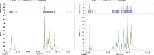
Table 7. Impact of the roof implementation on each of the sub-catchment where flat roofs are present. Abbreviations: Subcatch.nr. – sub-catchment number, Imperv – imperviousness; Highlighting: bold – peak reduction larger and equal 20%, italics + underlined – peak reduction lower and equal 10%

Subcatch nr.	Total Area	Roof Area	Roofs	Imperv	Slope	Original Peak Runoff	Peak Runoff with Green/GreyRoofs	Peak reduction
	[m^2]	[m^2]	[%]	[%]	[%]	[L/s]	[L/s]	[%]
2	5154	1561	30%	65%	6%	8.8	7.0	21%
3	5095	1151	23%	50%	13%	9.8	8.4	15%
4	6933	846	12%	47%	16%	13.9	12.7	9%
6	2527	1070	42%	65%	11%	9.2	6.3	32%
8	3059	1065	35%	60%	10%	6.1	4.8	22%
9	769	240	31%	56%	5%	2.0	1.6	20%
10	6073	763	13%	47%	16%	12.5	11.5	8%
12	3221	245	8%	44%	8%	6.4	6.1	4%
13	19,459	3199	16%	36%	14%	25.6	23.0	10%
14	1936	725	37%	64%	9%	7.0	5.0	28%
19	4916	838	17%	54%	14%	11.0	9.7	12%
20	2425	698	29%	55%	11%	5.9	4.8	19%
21	1107	33	3%	58%	9%	2.7	2.7	2%
22	1705	475	28%	41%	11%	4.5	3.5	22%
26	3600	729	20%	58%	11%	6.9	6.1	12%
28	1974	714	36%	65%	12%	6.1	4.6	24%
29	2095	541	26%	49%	8%	4.0	3.3	18%
30	2572	712	28%	61%	5%	4.5	3.6	20%
31	5336	1312	25%	54%	7%	9.5	8.2	14%
33	3954	123	3%	26%	24%	6.0	5.9	2%
34	7441	18	0%	6%	14%	0	0.1	0%
37	4416	1345	30%	52%	6%	6.6	5.3	20%
38	5167	645	12%	11%	19%	3.8	3.4	10%
44	2793	706	25%	38%	10%	5.1	4.3	16%
45	8519	2312	27%	49%	9%	15.2	12.5	17%
Min	769	18	0%	6%	5%	0	0	0%
Mean	4490	883	22%	48%	11%	7.7	6.6	15%
Median	3600	725	25%	52%	11%	6.4	5.3	16%
Max	19,459	3199	42%	65%	24%	25.6	23.0	32%

Figure A1. Climate data in 2017, maximum and minimum daily temperature, and wind speed records

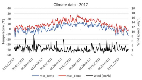
Figure A2. Climate data in 2018, maximum and minimum daily temperature, and wind speed records

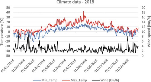
Table A1. Sensitivity analysis of 17 parameters for the whole period andwarm period with individual parameter adjustment by ±10% and ±50%

Table A2. Impact of the green and grey roofs downstream implementation for different exceedance thresholds 100, 50, and 25 L/s with respect to the evaluation criteria. Scenario A, F and G from Table 2

Evaluation criteria	Do nothing – Scenario A	GreenRoofs performance – Scenario F	GreyRoofs performance – Scenario G	Impact of GreenRoofs	Impact of GreyRoofs
Maximum Flow [L/s]	174	166	166	4%	4%
Exceedance threshold [L/s]	Duration of Exceedances [h]			Impact of GreenRoofs	Impact of GreyRoofs
100	1.4	1.4	1.2	−4%	13%
50	20	21	18	−5%	8%
25	118	121	112	−3%	5%
Exceedance threshold [L/s]	Number of Exceedances			Impact of GreenRoofs	Impact of GreyRoofs
100	8	9	9	−13%	−13%
50	67	71	63	−6%	6%
25	214	216	215	−1%	0%
Exceedance threshold [L/s]	Volume of Exceedances [m3]			Impact of GreenRoofs	Impact of GreyRoofs
100	132	114	106	14%	20%
50	1323	1317	1146	0%	13%
25	6046	6112	5573	−1%	8%

Table A3. Impact of the green and grey roofs upstream implementation for different exceedance thresholds 100, 50, and 25 L/s with respect to the evaluation criteria. Scenario A, H and I from Table 2

Evaluation criteria	Do nothing – Scenario A	GreenRoofs performance – Scenario H	GreyRoofs performance – Scenario I	Impact of GreenRoofs	Impact of GreyRoofs
Maximum Flow [L/s]	174	158	158	9%	9%
Exceedance threshold [L/s]	Duration of Exceedances [h]			Impact of GreenRoofs	Impact of GreyRoofs
100	1.4	1.2	0.9	13%	32%
50	20	20	15	2%	23%
25	118	114	100	3%	15%
Exceedance threshold [L/s]	Number of Exceedances			Impact of GreenRoofs	Impact of GreyRoofs
100	8	9	7	−13%	13%
50	67	69	58	−3%	13%
25	214	206	202	4%	6%
Exceedance threshold [L/s]	Volume of Exceedances [m3]			Impact of GreenRoofs	Impact of GreyRoofs
100	132	83	76	37%	42%
50	1323	1140	894	14%	32%
25	6046	5596	4758	7%	21%