Assessment of the suitability of degradation models for the planning of CCTV inspections of sewer pipes

Figures & data

Table 1. List of reviewed research papers, including the explanatory factors and the techniques used to model the degradation of sewer pipes.

Authors	Explanatory variables	Models
Mashford et al. (2011)	Diameter, age, road class, slope, Up/down invert elevation, material, grade, angle, soil corrosivity, sulfate soil/groundwater	Support Vector Machine
Salman and Salem (2012)	Size, length, slope, age, depth, road class, material, sewer function	Logistic Regression
Sousa et al. (2014)	Material, diameter, length, depth, slope, age, flow velocity	Logistic Regression
		Support Vector Machines
		Artificial Neural Networks
Sousa et al. (2019)	Material, diameter, sewer reaches, length, age, depth, slope, flow velocity	Support Vector Machines
		Artificial Neural Networks
Kabir et al. (2018)	Age, diameter, length, slope, depth, rim elevation, up and down invert	Bayesian Logistic Regression
Robles-Velasco et al. (2021)	Age, diameter, length, sewer function, soil type, shape, exposure to hydrogen sulphide, number of previous failures	Logistic Regression
Harvey and McBean (2014)	Material, age, installation era, type of sewer, diameter, length, slope, slope change, up and down invert elevation, orientation change, depth, road coverage, watermain breaks, land use, census tract	Random Forest Classifier
Laakso et al. (2019)	Slope, sewage flow, age, length, build year, coordinates, construction class, diameter, distance to trees, pipe type, material, depth, road class, stormwater pipe intersection, waterpipe intersection	Logistic Regression Random Forest
Hansen et al. (2020)	Size, material, pipe function, land use, previous rehabilitations, distance to buildings, distance to trees, soil type, road class, position, slope, groundwater level	Random Forest
Caradot et al. (2018)	Age, material, shape, effluent type, district, length, width, depth, soil type, groundwater level, backwater, distance to trees	Random Forest
Tran et al. (2006)	Size, age, depth, slope, tree-count, hydraulic condition, location, soil type, moisture index	Artificial Neural Network
Khan et al. (2010)	Length, diameter, material, age, bedding material, depth	Artificial Neural Network
Xianfei et al. (2020b)	Waste type, diameter, length, slope, water flow capacity, history of repairs, pipe function, material, age	Artificial Neural Network
Xianfei et al. (2020a)	Age, diameter, length, material, slope, average neighborhood LOF, Waste type, Up/down stream depth, repair history, Up/down invert elevation, water flow capacity, pipe function	Artificial Neural Network
Mohammadi et al. (2020)	Age, material, diameter, depth, slope, length, soil type, soils sulfate, soil pH, groundwater level, soil hydraulic group, soil corrosivity, water flow	Gradient Boosting Trees
Fontecha et al. (2021)	Weather, population, previous failures, elevation, land use, slope, number of trees, gully pots, manholes, sewer pipes, streets, type of pipeline (local/main), pipe function (stormwater/sanitary)	Logistic Regression Logistic Regression Random Forest Gradient Boosting Trees

Table 2. Main statistics of the numerical predictors.

Variable	Min.	Max.	Mean	SD
Age	0	74	30.199	16.705
Length	1.43	175.27	34.082	16.190
Size	100	2500	399.905	259.854
Depth	0.394	7.22	2.316	0.924
Slope	−0.309	67.333	0.979	2.177
Connection surface	0.568	1263.832	170.077	113.118
Upstream length	1.876	72009.122	1812.761	6205.549
Coordinates (X)	0	1	0.348	0.1466
Coordinates (Y)	0	1	0.547	0.219

Table 3. Input variables considered for the development of the model.

Variable name	Type	Description
Age	Numerical	Time elapsed between installation of the pipe and the inspection in years
Length	Numerical	Length of the pipe segment in meters
Size	Numerical	Height of the pipe segment in millimeters
Depth	Numerical	Average depth of the pipe segment in meters
Slope	Numerical	Slope of the pipe segment in percentage
Connection surface	Numerical	Surface of the connection between the pipe and the manholes in squared meters
Upstream length	Numerical	Length of the upstream pipes in meters
Upstream pipes	Numerical	Count of upstream pipes
Coordinates	Numerical	X and Y Geographical coordinates of the centroid of the pipe, expressed in degrees
Material	Categorical	Material of the pipe segment
Waste type	Categorical	Type of waste conducted by the pipe (wastewater, stormwater, mixed)

Figure 1. a) box plot showing the distribution of pipe age within damage classes. b) count of inspections that fall within each damage class.

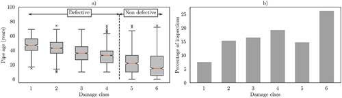
Figure 2. Descriptive statistics of the main variables considered for the development of the model. (VC: vitrified clay, PP: polypropylene, CI: cast iron, PVC: polyvinyl chloride, PRC: polymer concrete, GRP: glass reinforced plastic, PE: polyethylene, PVCU: unplasticised PVC).

Figure 3. Flowchart of the proposed methodology.

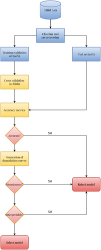
Figure 4. Cross-validated accuracy scores of the models on the held-out test set.

Figure 5. Degradation curves showing the probability of failure of four different sewer pipes according to the trained models.

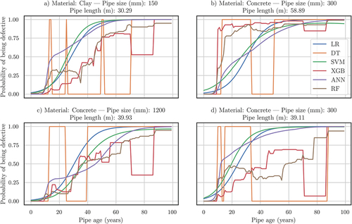
Table 4. Comparison of the average performance metrics (and standard deviation) of the tested models. Random Forest yields the best results for all the metrics.

Model	Accuracy	Recall	Precision	AUC
LR	76.995 (0.254)	81.921 (0.595)	78.721 (0.321)	0.849 ($9.59\times {10}^{-4}$)
DT	76.704 (0.998)	80.904 (1.229)	78.908 (1.047)	0.759 ($1.045\times {10}^{-2}$)
SVM	77.657 (0.544)	89.039 (0.921)	76.014 (0.652)	0.863 ($1.926\times {10}^{-3}$)
XGB	82.827 (1.063)	90.734 (1.317)	81.382 (0.873)	0.898 ($4.995\times {10}^{-3}$)
ANN	77.689 (0.763)	86.779 (3.244)	77.185 (1.893)	0.869 ($6.576\times {10}^{-3}$)
RF	83.311 (0.533)	91.356 (1.058)	81.666 (1.023)	0.911 ($3.455\times {10}^{-3}$)

Table 5. Metrics of the models in terms of the monotonicity of the degradation curves compared across every sample in the dataset.

Model	Count	Mean	Max
LR	0	0	0
DT	8,224	1.33	4
SVM	16,504	2.67	14
XGB	44,033	7.12	15
ANN	0	0	0
RF	54,593	8.82	24

Table 6. Coefficient estimates, significance and Odds ratios of the variables used in the Logistic Regression model.

	Coefficients					Odds Ratio
Variable	Estimate	Std. error	z value	P($>$$|\mathit{z}|$)	Significance	Estimate	CI 2.50%	CI 97.50%
Pipe age	9.141$\times {10}^{-2}$	2.795$\times {10}^{-3}$	32.706	$<$$2\times {10}^{-16}$	***	1.095	1.089	1.101
Upstream length	$2.818\times {10}^{-2}$	$6.367\times {10}^{-3}$	4.426	$7.391\times {10}^{-6}$	***	1.028	1.016	1.041
Pipe length	$9.915\times {10}^{-3}$	$3.212\times {10}^{-3}$	3.087	$2.024\times {10}^{-3}$	**	1.009	1.003	1.016
Pipe size	−1.527	0.183	−8.310	$<$ $2\times {10}^{-16}$	***	0.217	0.151	0.312
Connection surface	$1.284\times {10}^{-3}$	$5.392\times {10}^{-4}$	2.381	$1.775\times {10}^{-2}$	*	1.001	1.000	1.002
Depth	$3.824\times {10}^{-2}$	$5.955\times {10}^{-2}$	0.642	0.521		1.038	0.924	1.167
Slope	$5.231\times {10}^{-3}$	$8.681\times {10}^{-3}$	0.603	0.546		1.005	0.987	1.024
Material
Asbestos	0.643	0.534	1.204	0.228		1.903	0.683	5.576
Concrete	0.216	0.412	0.524	0.600		1.241	0.562	2.851
CI	−4.469	0.481	−9.275	$<$ $2\times {10}^{-16}$	***	$1.146\times {10}^{-2}$	$4.484\times {10}^{-3}$	$2.977\times {10}^{-2}$
PE	−13.882	$2.854\times {10}^2$	$-4.924\times {10}^{-2}$	0.961		$9.372\times {10}^{-7}$	$4.523\times {10}^{-135}$	$3.787\times {10}^{-115}$
PP	−2.043	0.602	−3.393	$6.983\times {10}^{-4}$	***	0.129	$3.828\times {10}^{-2}$	0.411
PRC	−13.623	19.703	$-6.928\times {10}^{-2}$	0.9448		$1.215\times {10}^{-6}$	$5.175\times {10}^{-102}$	$8.901\times {10}^{-89}$
PVC	−0.845	0.476	−1.773	$7.623\times {10}^{-2}$	.	0.429	0.171	1.110
PVCU	−0.549	0.739	−0.743	0.457		0.577	0.126	2.356
Clay	−0.199	0.427	−0.468	0.640		0.818	0.361	1.934
Sewer type
Combined sewer	$8.704\times {10}^{-2}$	$9.129\times {10}^{-2}$	0.952	0.341		1.091	0.912	1.305
Stormwater	−0.359	0.126	−2.858	$4.271\times {10}^{-3}$	**	0.698	0.545	0.893
Coordinates
X	−10.2	1.542	−6.611	$3.812\times {10}^{-11}$	***	$3.741\times {10}^{-5}$	$1.803\times {10}^{-6}$	$7.620\times {10}^{-4}$
Y	1.432	0.226	6.435	$1.241\times {10}^{-10}$	***	4.187	2.710	6.487

‘***’: p$<$0.001; ‘**’: p$<$0.01; ‘*’: p$<$0.05; ‘’.: p$<$ 0.1.

Figure 6. The map shows the density of population of the area under study, represented by the approximated count of inhabitants in each pixel. The color of the pipes represent the probability of failure at age 20 of each pipe. Pipes located in the upper left part of figure show a higher probability of failure than the ones located in the opposite side of the area under study. Population density map provided by WorldPop tatem (2017) worldpop.

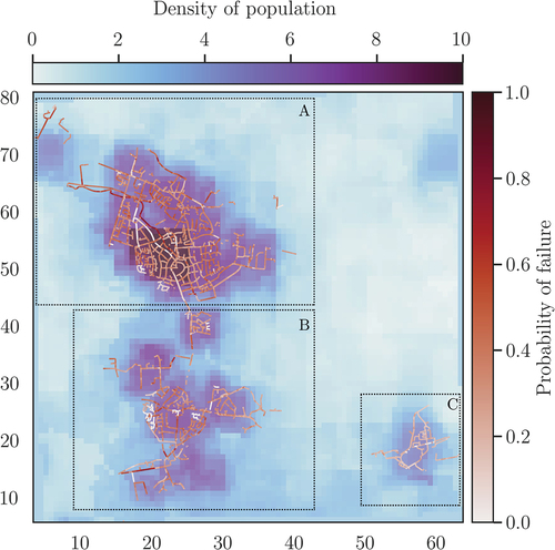
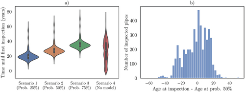
Figure 7. a) comparison of alternative scenarios considering different probability thresholds with the current scenario b) difference of pipe ages at inspection between the current strategy and the results of a model with a probability threshold of 50%.

Mashford, J., D. Marlow, D. H. Tran, and R. May. 2011. “Prediction of Sewer Condition Grade Using Support Vector Machines.” Journal of Computing in Civil Engineering 25 (4): 283–290. https://doi.org/10.1061/(asce)cp.1943-5487.0000089.

 Web of Science ®Google Scholar

Salman, B., and O. Salem. 2012. “Modeling Failure of Wastewater Collection Lines Using Various Section-Level Regression Models.” Journal of Infrastructure Systems 18 (2): 146–154. https://doi.org/10.1061/(ASCE)IS.1943-555X.0000075.

 Web of Science ®Google Scholar

Sousa, V., J. P. Matos, and N. Matias. 2014. “Evaluation of Artificial Intelligence Tool Performance and Uncertainty for Predicting Sewer Structural Condition.” Automation in Construction 44:84–91. https://doi.org/10.1016/J.AUTCON.2014.04.004.

 Web of Science ®Google Scholar

Sousa, V., J. P. Matos, N. Matias, and I. Meireles. 2019. “Statistical Comparison of the Performance of Data-Based Models for Sewer Condition Modeling.” Structure and Infrastructure Engineering 15 (12): 1680–1693. https://doi.org/10.1080/15732479.2019.1648525.

 Web of Science ®Google Scholar

Kabir, G., N. B. C. Balek, and S. Tesfamariam. 2018. “Sewer Structural Condition Prediction Integrating Bayesian Model Averaging with Logistic Regression.” Journal of Performance of Constructed Facilities 32 (3): 04018019. https://doi.org/10.1061/(ASCE)CF.1943-5509.0001162.

 Web of Science ®Google Scholar

Robles-Velasco, A., P. Cortés, J. Muñuzuri, and L. Onieva. 2021. “Estimation of a Logistic Regression Model by a Genetic Algorithm to Predict Pipe Failures in Sewer Networks.” OR Spectrum 43 (3): 759–776. https://doi.org/10.1007/s00291-020-00614-9.

 Web of Science ®Google Scholar

Harvey, R. R., and E. A. McBean. 2014. “Predicting the Structural Condition of Individual Sanitary Sewer Pipes with Random Forests.” Canadian Journal of Civil Engineering 41 (4): 294–303. https://doi.org/10.1139/cjce-2013-0431.

 Web of Science ®Google Scholar

Laakso, T., T. Kokkonen, I. Mellin, and R. Vahala. 2019. “Sewer Life Span Prediction: Comparison of Methods and Assessment of the Sample Impact on the Results.” Water 11 (12): 1–14. https://doi.org/10.3390/W11122657.

 Web of Science ®Google Scholar

Hansen, B. D., S. H. Rasmussen, T. B. Moeslund, M. Uggerby, and D. G. Jensen. 2020. “Sewer Deterioration Modeling: The Effect of Training a Random Forest Model on Logically Selected Data-Groups.” Procedia Computer Science 176:291–299. https://doi.org/10.1016/j.procs.2020.08.031.

 Google Scholar

Caradot, N., M. Riechel, M. Fesneau, N. Hernandez, A. Torres, H. Sonnenberg, E. Eckert, N. Lengemann, J. Waschnewski, and P. Rouault. 2018. “Practical Benchmarking of Statistical and Machine Learning Models for Predicting the Condition of Sewer Pipes in Berlin, Germany.” Journal of Hydroinformatics 20 (5): 1131–1147. https://doi.org/10.2166/hydro.2018.217.

 Web of Science ®Google Scholar

Tran, D. H., A. W. Ng, B. J. Perera, S. Burn, and P. Davis. 2006. “Application of Probabilistic Neural Networks in Modelling Structural Deterioration of Stormwater Pipes.” Urban Water Journal 3 (3): 175–184. https://doi.org/10.1080/15730620600961684.

 Google Scholar

Khan, Z., T. Zayed, and O. Moselhi. 2010. “Structural Condition Assessment of Sewer Pipelines.” Journal of Performance of Constructed Facilities 24 (2): 170–179. https://doi.org/10.1061/(asce)cf.1943-5509.0000081.

 Web of Science ®Google Scholar

Xianfei, Y., Y. Chen, A. Bouferguene, M. Al-Hussein, R. Russell, and L. Kurach. 2020. “A Neural Network-Based Approach to Predict the Condition for Sewer Pipes.” Construction Research Congress 7:809–818. https://doi.org/10.1061/9780784482858.017.

 Google Scholar

Xianfei, Y., Y. Chen, A. Bouferguene, and M. Al-Hussein. 2020. “Data-driven bi-level sewer pipe deterioration model: Design and analysis.” Automation in Construction 116:116. https://doi.org/10.1016/j.autcon.2020.103181.

 Web of Science ®Google Scholar

Mohammadi, M. M., M. Najafi, N. Salehabadi, R. Serajiantehrani, and V. Kaushal. 2020. Predicting Condition of Sanitary Sewer Pipes with Gradient Boosting Treepp. 80–89. American Society of Civil Engineers. https://doi.org/10.1061/9780784483206.010.

 Google Scholar

Fontecha, J. E., P. Agarwal, M. N. Torres, S. Mukherjee, J. L. Walteros, and J. P. Rodríguez. 2021. “A Two-Stage Data-Driven Spatiotemporal Analysis to Predict Failure Risk of Urban Sewer Systems Leveraging Machine Learning Algorithms.” Risk Analysis 41 (12): 2356–2391. https://doi.org/10.1111/risa.13742.

 PubMed Web of Science ®Google Scholar

Tatem, A. J. 2017. “Worldpop, Open Data for Spatial Demography.” Scientific Data 4 (1): 1–4. https://doi.org/10.1038/sdata.2017.4.

 Google Scholar

Data availability statement

The data used in this study are available upon request from the corresponding author or can be accessed through the following GitHub repository: https://github.com/Fidaeic/sewer-pred.