Figures & data
Figure 2. Procedure for analysis of spatial blockage data. References to the corresponding Sections where the methods are elaborated have been added.
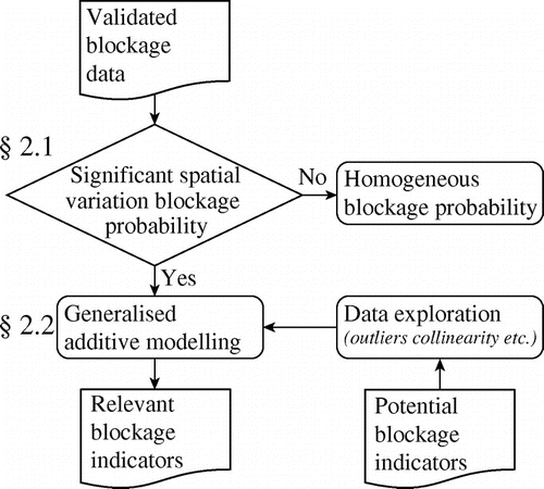
Figure 3. Example of the cross section of a bivariate kernel density function at coordinates s, given by the sum of n kernels at coordinates S1, Si, … Sn coordinates and bandwidth h.
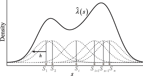
Table 1. Characteristics of Rotterdam and The Hague city examples.
Figure 4. Distribution of the observed failure mechanisms: incorrect use (e.g. sanitary towels, kitchen waste etc.), structural defect, deposit build up for both the full data-set and the analysed subset. Error bars represent 95% bootstrap confidence intervals.
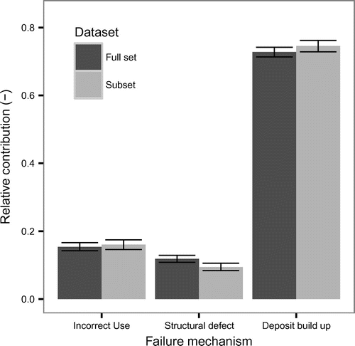
Table 2. Factors that may indicate an increase in the likelihood of a blockage.
Figure 5. Shape of the likelihood based cross validation (CV) function 2–3 for the bandwidth h of the kernel density function 2–2. Vertical grey lines show the optimum values.
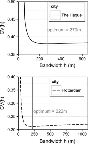
Figure 6. Kernel ratio of the intensity of blockages for Rotterdam (left panel) and The Hague (right panel). Dark colours denote regions with a high blockage intensity. White dashed lines and black dashed lines indicate the 97.5% and 2.5% Monte Carlo simulation contours respectively. P-values for both Rotterdam (0.001) and The Hague (0.004) provided evidence to reject the hypothesis of a constant blockage intensity for the city.
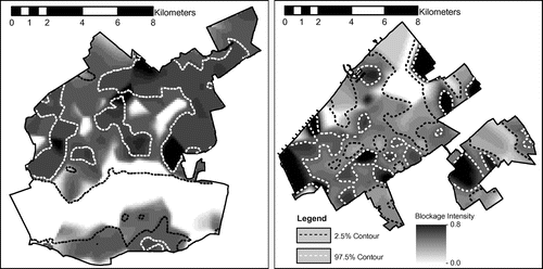
Figure 7. Empirical cumulative distribution function of the standardised regression weights β for each factor for The Hague that is significantly different from 0, based on 50,000 bootstrap samples. The 95% confidence interval is depicted by the grey area. Factors are considered significantly different from zero, when the dashed vertical line at β = 0 is not contained within the 95% confidence interval.
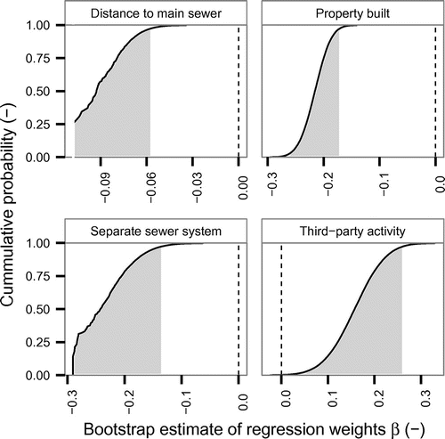
Table 3. Median estimate of the standardised regression weights β for each factor for The Hague that is significantly different from 0. The 95% confidence intervals are in parentheses.
Figure 8. Correlation matrix of the regression weights β for each significant factor for The Hague, based on 50,000 bootstrap samples. Triangles indicate the strength and direction of the correlation.
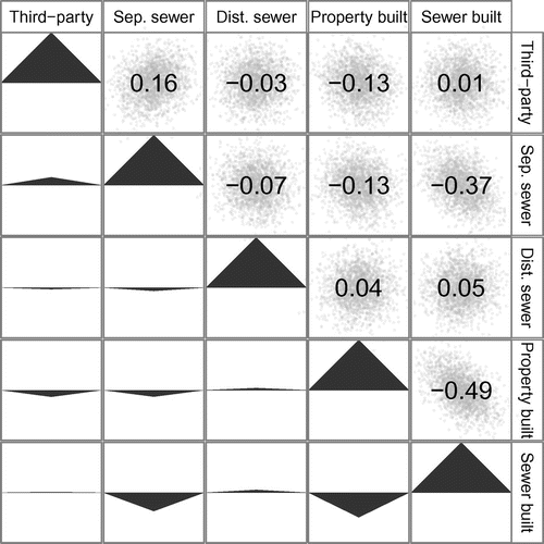
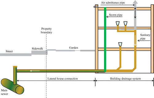
Figure 9. Boxplot of the garden lengths, used to approximate the length of the lateral house connection on private ground.
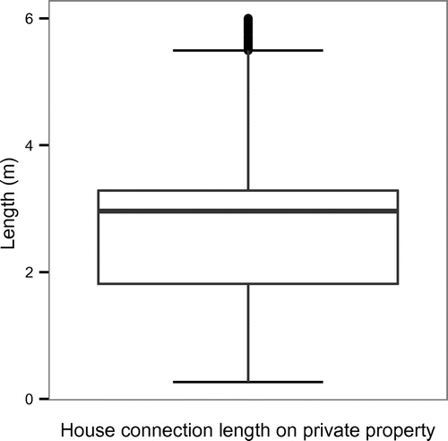
Figure 10. Empirical cumulative distribution function of the standardised regression weights β for each factor for Rotterdam that is significantly different from 0, based on 50,000 bootstrap samples. The 95% confidence interval is depicted by the grey area. Factors are considered significantly different from zero, when the dashed vertical line at β = 0 is not contained within the 95% confidence interval.
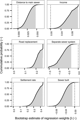
Table 4. Median estimate of the standardised regression weights β for each factor for Rotterdam that is significantly different from 0. The 95% confidence intervals are in parentheses.
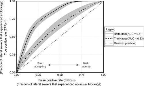
Figure 11. Receiver operating characteristic (ROC) curves for both The Hague and Rotterdam, illustrating the trade-off between the true positive rate and the false positive rate. Grey areas correspond to the 95% confidence interval. The Area Under the Curve (AUC) is a measure of the overall model performance.
