Variable mass loading effect on the long-term ambient response of a freeway bridge

Figures & data

Figure 1. Aerial photograph of the Lueg bridge (Brenner Autobahn AG, 1972).

Figure 2. Longitudinal and cross-section of the Lueg bridge (Brenner Autobahn AG, 1972), acceleration sensor location marked.

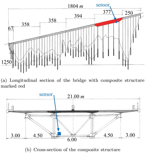
Figure 3. Number of all crossing vehicles and trucks per day recorded near the Lueg bridge in 2008.

Figure 4. Daily ambient mean temperature recorded near the Lueg bridge in 2008.

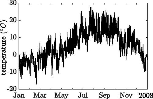
Figure 5. Auto spectral density of the three acceleration components for two different periods of time.

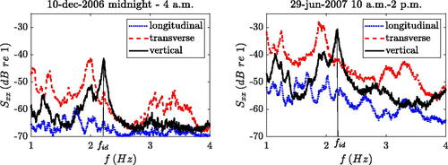
Figure 6. Time-frequency analysis of acceleration signals.

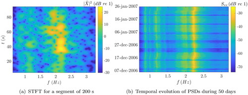
Figure 7. Variation of the identified resonance frequency in three 50 day periods of three subsequent years.

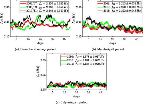
Figure 8. Identified resonance frequency and ambient temperature in two 50 day periods.

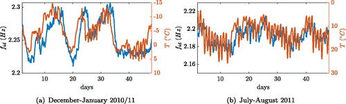
Figure 9. Daily distribution of total traffic volume with relation to the time of day.

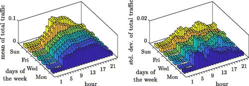
Figure 10. Daily quantity of trucks as a function of vehicle mass.

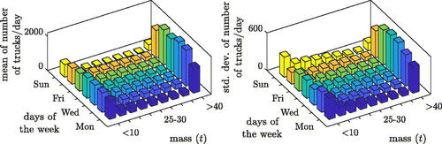
Figure 11. Statistics on the daily quantity of trucks as a function of month.

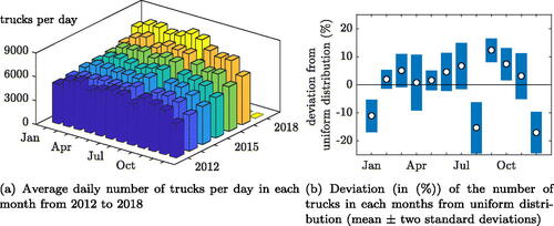
Figure 12. FE simulation for derivation of equivalent beam stiffness parameters.

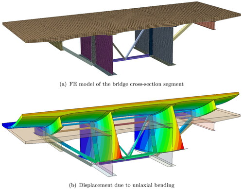
Table 1. Equivalent beam stiffness parameters for unit deformations of the bridge cross-section segment.

Torsional stiffness	GIt	=	$1.48·{10}^{11} N{m}^2$
Bending stiffness (vertical axis)	EIy	=	$8.51·{10}^{12} N{m}^2$
Bending stiffness (horizontal axis)	EIz	=	$4.35·{10}^{11} N{m}^2$
Transverse shear stiffness (vertical axis)	GAy	=	$1.12·{10}^{10} N$
Transverse shear stiffness (horizontal axis)	GAz	=	$7.41·{10}^{10} N$

Figure 13. Mechanical model of the bridge with truck crossing and location of the acceleration sensor.

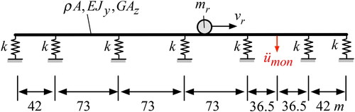
Figure 14. Mode shapes for natural frequencies f₂, f₄ and f₆ of the FE model using 2D beam elements.

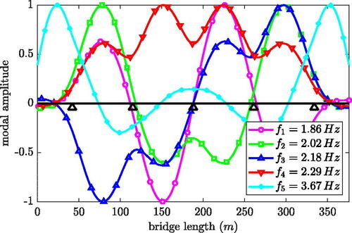
Table 2. Natural frequencies and participation factors for the first five modes of the 2D FE model.

Mode no. I	1	2	3	4	5
Natural frequency fi (Hz)	1.85	2.01	2.18	2.29	3.66
Participation factor Li	0.00	0.26	0.00	1.06	0.54

Table 3. Random variables (RV) for the stochastic simulation of truck traffic.

RV	Dimension	Distribution	Assignment
${\mathbf{y}}_1$	9	Normal	Number of trucks of each mass class
${\mathbf{y}}_2$	24	Normal	Distribution of trucks per hour
${\mathbf{y}}_3$	Variable	Uniform	Mass of each truck
y4	1	Normal	Velocity of the truck
y5	1	Uniform	Arrival time of truck within one hour
y6	1	Uniform	Length of the truck

Figure 15. Accelerations at monitor node ${\ddot{u}}_{\mathit{mon}}$ and instantaneous frequency f_sim from time-history analysis of one week truck traffic.

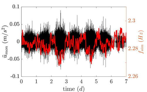
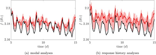
Figure 16. Change of resonance frequency with respect to reference value $f_{\mathit{ref}}=2.29 Hz$ (mean value μ, standard deviation σ) for two percentages of convoys, from modal analyses. 100 weeks observation time.

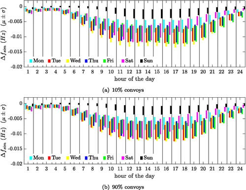
Figure 17. Change of resonance frequency with respect to reference value $f_{\mathit{ref}}=2.29 Hz$ (mean value μ, standard deviation σ) for (a) 10% and (b) 90% of all trucks in convoys, from response history analyses. 100 weeks observation time.

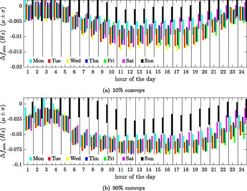
Table 4. Relative change in % of standard deviation of the identified resonance frequency over 50 days due to mass compensation (compare with Figure 7).

Period		Modal analyses		Response history analyses
		10%	90% convoys	10%	90% convoys	90%, scale 1/7
	2006/07	+1.5	+1.1	+1.8	+87.4	+2.2
Dec/Jan	2008/09	+0.3	+0.2	+0.5	+24.9	+0.5
	2010/11	+0.1	+0.0	+0.1	+28.8	+0.2
	2008	−5.0	−4.8	−4.6	+44.1	−4.1
Mar/Apr	2010	−3.5	−3.7	−3.3	+60.2	−2.9
	2011	−3.2	−3.0	−3.1	+19.1	−2.8
	2009	−8.3	−8.1	−8.0	+131.3	−5.5
Jul/Aug	2010	−8.7	−8.4	−8.7	+80.8	−8.0
	2011	−11.2	−10.7	−11.8	+87.9	−9.5

Figure 18. Identified resonance frequency time-history for 10 days in July 2011 (black), mass-compensated time-histories (mean values in red including 95% confidence interval).

Brenner Autobahn AG. (1972). The brenner motorway (in German). Innsbruck, Austria: Verlag Tiroler Nachrichten.

 Google Scholar