The practical value of structural health information for time dependence in bridge maintenance

Figures & data

Figure 1. Influence diagram for the fundamental decision case, from Björnsson et al. (2019).

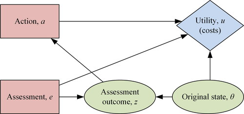
Figure 2. Decision tree for the fundamental case, related to the influence diagram in Figure 1 and Equations 1(1) $$u^{\mathrm{*}}=ma{x}_e(\sum _{z\in Z}P\left(z|e\right)·(ma{x}_a\left(\sum _{\theta \in \mathrm{\Theta }}u\left(e,\stackrel{\sim }{z},a,\stackrel{\sim }{\theta }\right)·P^{\text{″}}\left(\theta |z\right)\right)\left)\right)$$(1) and 2(2) $$ma{x}_a\left(E\right[u\left(a|e,\stackrel{\sim }{z}\right)]=ma{x}_a(\sum _{\theta \in \mathrm{\Theta }}u(e,\stackrel{\sim }{z},a,\stackrel{\sim }{\theta })·P^{\text{″}}\left(\theta |z\right)\left)\right)$$(2) , from Björnsson et al. (2019).

Table 1. Condition classes in the Swedish bridge management system (Trafikverket, 2015).

Condition class	Estimated consequence
CC0	Lack of function beyond 10 years
CC1	Lack of function within 10 years
CC2	Lack of function within 3 years
CC3	Lack of function at time of inspection

Figure 3. Schematic representation on the degree of degradation dependence on time, with uncertainty represented by distribution around the degradation curve, for a section of the lifetime for a structure.

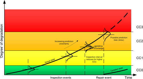
Figure 4. Updated influence diagram for the extended fundamental case (original influence diagram can be found in Figure 1).

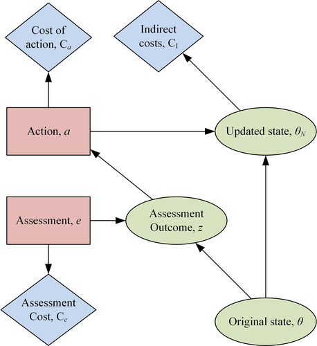
Figure 5. Extended influence diagram to incorporate time aspects such as updates in bridge state and benefits for the overall bridge stock if do nothing is chosen at the first decision point (extended from Figures 1 and 4), where t₂ occurs after t₁.

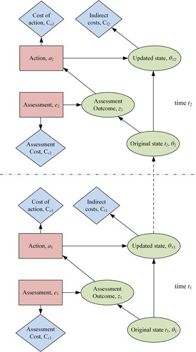
Figure 6. Picture of the bridge with details of the damaged column (bottom left) and damaged edge beam (bottom right), courtesy of the Swedish Transport Administration.

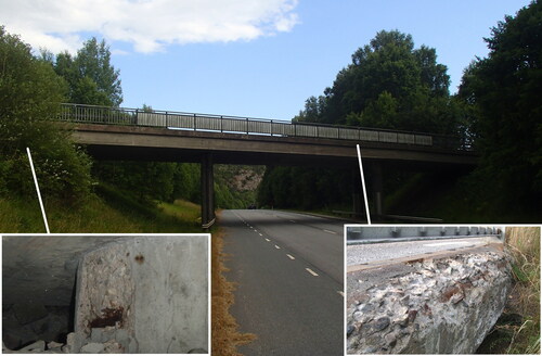
Table 2. Results from routine inspection.

Bridge part	Condition Class	Inspection result	Limit for CC3	Measurement procedure
Edge beam – weathering	3	20 %	20%	Loss in bond capacity
Edge beam – steel lining	3	4	4	Level of visible corrosion (4 means 8-40 % visible rust)
Column – corrosion rebars	2	5 %	20%	Loss in reinforcement area

Table 3. Distribution of probability of original state in a specific condition class.

Condition class	Probability (%)
CC0	0
CC1	10
CC2	45
CC3	45

Table 4. Costs used in the study.

	Cost (€)
Assessment methods
Desktop evaluation	10 000
Measurements	70 000
Repair Costs	750 000
Indirect Costs (CC3)	1000 000

Table 5. Sample likelihoods, z, used for the assessment methods.

	Desktop evaluation				Measurements
Assessment result, z	True state				True state
	CC0	CC1	CC2	CC3	CC0	CC1	CC2	CC3
CC0	0.7	0.15	0	0	0.95	0.025	0	0
CC1	0.3	0.7	0.15	0	0.05	0.95	0.025	0
CC2	0	0.15	0.7	0.3	0	0.025	0.95	0.05
CC3	0	0	0.15	0.7	0	0	0.025	0.95

Table 6. Probabilities of updated state after action is chosen, including probability of degradation if “Do nothing” is the chosen action.

	Do nothing				Replace beams
New State	Original state				Original state
	CC0	CC1	CC2	CC3	CC0	CC1	CC2	CC3
CC0	0.9	0	0	0	1	1	1	1
CC1	0.1	0.8	0	0	0	0	0	0
CC2	0	0.2	0.7	0	0	0	0	0
CC3	0	0	0.3	1	0	0	0	0

Figure 7. Point-in-time decision model as illustrated in Figure 4, with actual inputs in the various nodes.

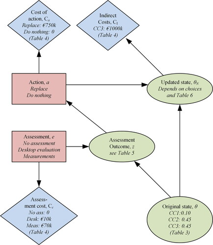
Figure 8. Sequential updating decision model as illustrated in Figure 5, with actual inputs in the various nodes.

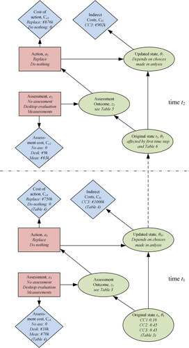
Table 7. Expected costs for the different assessments using point-in-time decision model and sequential updating decision model. (€).

	Point-in-time decision model	Sequential updating decision model
Assessment	Expected costs	Expected costs
Desktop evaluation	546 600	681 200
Measurement	553 200	649 000
No assessment	585 000	750 000

Table 8. Expected costs for the two possible actions using point-in-time decision model and sequential updating decision model, related to the two available assessment methods.

		Point-in-time decision model		Sequential updating decision model
Assessment result		Do nothing	Replace	Do nothing	Replace
Desktop evaluation	CC0	10 000	760 000	64 000	760 000
	CC1	157 300	760 000	263 000	760 000
	CC2	503 600	760 000	875 500	760 000
	CC3	886 500	760 000	1510 000	760 000
Measurements	CC0	70 000	820 000	124 100	820 000
	CC1	101 800	820 000	167 100	820 000
	CC2	403 100	820 000	599 400	820 000
	CC3	1052 000	820 000	1720 800	820 000

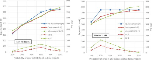
Figure 9. Relation between expected costs (left y-axis) for the assessment options and the likelihood of the edge beams being in CC3 for point-in Time model (left) and sequential updating model (right), with a relation CC2/CC1 of 4.5; along with the Value of Information (VoI; right y-axis) of the two assessment options (desktop evaluation (B) and measurements (C)), defined as the difference between expected costs for no assessment and the expected costs for the respective assessment option, minus the cost of the assessment method.

Björnsson, I., Larsson Ivanov, O., Honfi, D., & Leander, J. (2019). Decision support framework for bridge condition assessments. Structural Safety, 81, 101874. doi:https://doi.org/10.1016/j.strusafe.2019.101874

 Web of Science ®Google Scholar

Trafikverket. (2015). BaTMan handbook (In Swedish). Swedish Transport Administration. https://batmanhandbok.trafikverket.se

 Google Scholar