A simplified method based on improved multiplication factors to assess crowd-induced vertical vibrations of footbridges

Figures & data

Figure 1. General framework of the procedure, with crowd densities ρ ranging from 0.2 to 1.5 ped/m², natural frequencies f from 0.5 to 5.5 Hz, and damping ratios ξ from 0.1 to 10%, which correspond to extra dampings ${\xi }^{*}$ in line with Section 6.1.

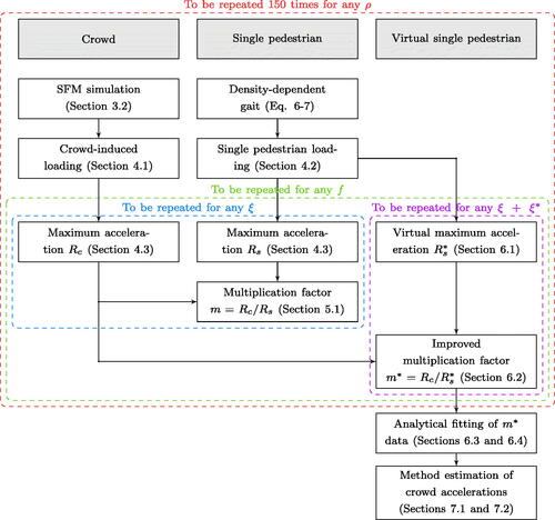
Figure 2. Example pedestrian crossing the footbridge: trajectory (black line), foot standing points on the trajectory (black markers), and projection of the foot positions on the bridge centreline (grey markers).

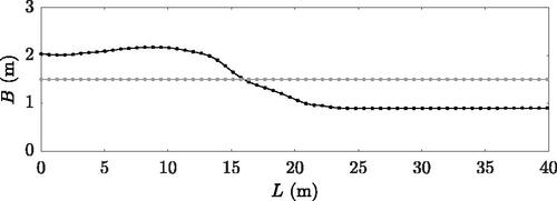
Table 1. Meta-parameters implemented in the SFM after Bassoli and Vincenzi (2021).

Model parameter	Value	References
${\tau }_{\alpha }$ (s)	0.5	Helbing & Molnár (1995)
$A_{\alpha i}$ (m/s^2)	5	Helbing et al. (2005)
$B_{\alpha i}$ (m)	0.1	Helbing et al. (2005)
$r_{\alpha }$ (m)	0.31	Bassoli & Vincenzi (2021)
${\lambda }_{\alpha }$ (-)	0.31	Bassoli & Vincenzi (2021)
$A_{\alpha ,1}$ (m/s^2)	1.7	Bassoli & Vincenzi (2021)
$B_{\alpha ,1}$ (m)	0.28	Bassoli & Vincenzi (2021)

Figure 3. SFM simulated crowd made of 108 pedestrians: instantaneous (a) number of occupants and (b) mean crowd velocity in thick black, respective theoretical values in thin grey.

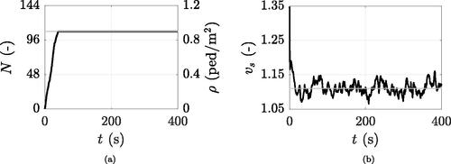
Figure 4. Standard deviation of personal simulated speeds (a) and step frequencies (b) versus crowd density.

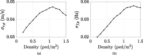
Figure 5. Standard deviation of collective speeds (a) and step frequencies (b) versus crowd density: simulations (dot markers) and analytical proposal (grey line).

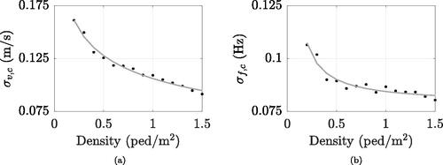
Figure 6. Implemented loadings: (a) force induced by a pedestrian who is part of a crowd (thick line), obtained by the superimposition of left (thin black lines) and right (thin grey lines) step forces; (b) force due to the crowd-coupled undisturbed representative single pedestrian; (c) modal force corresponding to (a); (d) modal force induced by the overall crowd.

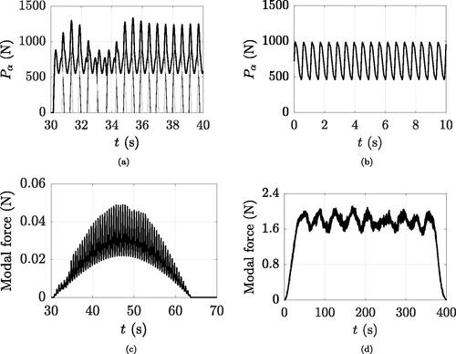
Figure 7. Example case of $\rho =0.9$ ped/m² and $\xi =0.5$%: (a) crowd-induced maximum accelerations (150 simulated runs) in black and mean trend in dashed white, (b) maximum acceleration due to the crowd-coupled single pedestrian, (c) multiplication factors in black and mean trend in dashed white.

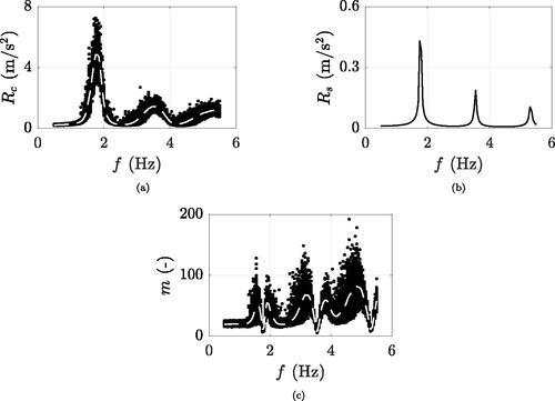
Figure 8. Simulated mean crowd-induced maximum acceleration (black) and 95% confidence intervals (grey) to increasing number of runs: $\rho =0.9$ ped/m², $\xi =0.5$% and (a) f = 1.77 Hz or (b) f = 3.54 Hz.

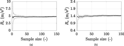
Figure 9. Standard deviation of numerically simulated crowd-induced accelerations, ${\sigma }_{R_c},$ varying one parameter individually while keeping all others constant at their example values: $\rho =0.9$ ped/m², $\xi =0.005$ (-), f = 1.77 (black lines) or 2.65 Hz (grey lines).

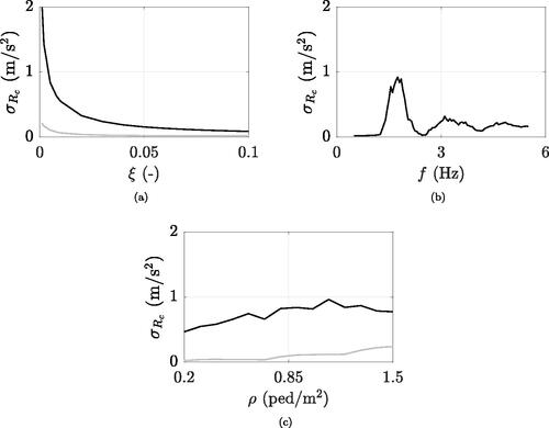
Figure 10. Simulated multiplication factor (in black) compared to the literature (Bachmann and Ammann (1987) in dashed red, Grundmann et al. (1993) in dash-dotted green, and Fujino et al. (1993) in dotted blue): (a) specific crowd density and structural damping ($\rho =0.9$ ped/m², $\xi =0.5$%), (b) fixed natural frequency depending on the crowd density.

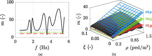
Figure 11. Example case of $\rho =0.9$ ped/m² and $\xi =0.5$%: (a) maximum acceleration due to the crowd-coupled virtual single pedestrian; (b-c) simulated improved multiplication factors in black, mean trend in dashed white, (b) fitted function in solid green, and (c) analytical function in solid blue; (d) simulated crowd induced maximum accelerations in black, mean trend in dashed white, and analytical prediction in solid blue.

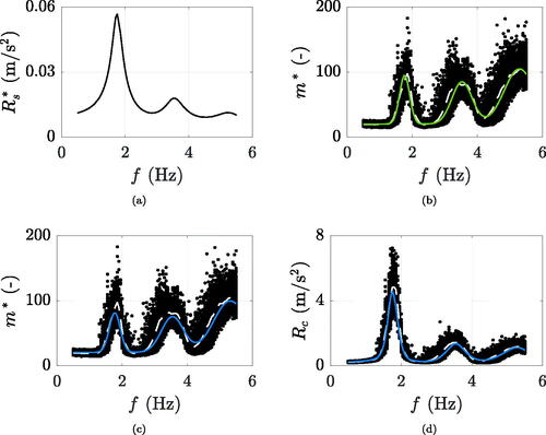
Figure 12. Analytical definition (blue surfaces) of two out of eight parameters, based on the discrete values resulting from the simulated improved multiplication factor mean trend fitting (green dots).

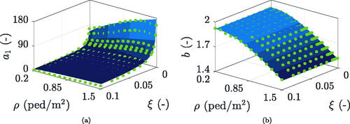
Table 2. Analytical definitions of coefficients a₁, a₂, a₃, b, c₁, c₂, c₃, and d. In this, f_s follows Equation (6)(6) $$v_s(\rho )=1.34\{1-\hspace{0.17em}\mathrm{\text{exp}}[-1.913(\frac{1}{\rho }-\frac{1}{5.4})\left]\right\}$$(6) and Equation (7)(7) $$f_{s,\alpha }(v_{s,\alpha })=0.35{(v_{s,\alpha })}^3-1.59{(v_{s,\alpha })}^2+2.93v_{s,\alpha }$$(7) adopted in sequence, ρ is expressed in ped/m², A in m², and ξ is unitless (-).

an	b	cn	d
$a_1=0.4105\sqrt{\rho A}{\xi }^{-0.5021}$	b = fs	$c_1=0.24$	$d=1.868\sqrt{\rho A}{\xi }^{-0.01086}$
$a_2=0.9a_1$		$c_2=2c_1$
$a_3=1.3a_1$		$c_3=3c_1$

Figure 13. Example case of $\rho =0.9$ ped/m² and $\xi =0.5$%: (a) simulated crowd induced maximum accelerations in black, 95th percentile in dash-dotted white, and analytical prediction in solid red; (b) analytical definition (red surface) of the Δ factor, based on the discrete values resulting from the ratio of 95th to 50th percentiles of simulated maximum crowd-induced accelerations (orange dots).

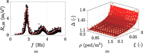
Figure 14. Method prediction of the accelerations R_c (average maximum) and $R_{c,95}$ (95th percentile maximum) induced by a crowd density $\overline{\rho }$ within $[0.2,1.5]$ ped/m² on a footbridge whose natural frequency $\overline{f}$ and damping ratio $\overline{\xi }$ are between $[0.5,5.5]$ Hz and $[0.001,0.1]$ (-), respectively. In case of considering HSI, replace $\overline{f}$ and $\overline{\xi }$ with the dynamic properties of the crowd-structure coupled system.

Figure 15. Overlay of crowd-induced maximum accelerations predicted by the method referring to (a) fixed damping ratio ($\xi =0.5$%) and varying crowd density, and (b) fixed crowd density ($\rho =0.9$ ped/m²) and varying damping ratio.

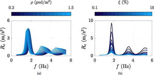
Figure 16. Crowd accelerations (maximum values) resulting from the post-processed SFM (black dots) and relevant mean trend (red line) for $\xi =0.5$% and f equal to (a) 1.5 and (b) 2.0 Hz.

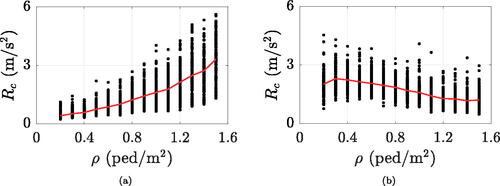
Figure 17. Example case of $\rho =0.9$ ped/m² and $\xi =0.5$%: overlay of crowd-induced maximum accelerations predicted by the method at varying (a) footbridge length L (m) and (b) footbridge width B (m).

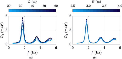
Figure 18. Maximum crowd accelerations: (i) simulated through the post-processed SFM (black dots) with corresponding 95th percentile (white dash-dot line), (ii) estimated by the method (red line), and (iii) induced by the guideline forcings (violet point markers, blue dashed, green dash-dot and grey dotted lines respectively correspond to BSI (2008), HIVOSS (2008), ISO 10137 (2007), and SETRA (2006)) for six representative density-damping clusters, combining crowd densities of 0.5, 0.8 and 1.0 ped/m² (in rows) to structural damping ratios of 0.5 and 1.0% (in columns).

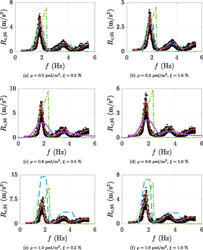
Table 3. Free walking events performed on the eeklo footbridge by Van Nimmen et al. (2021): identification names, crowd densities, experimental maximum accelerations at the mid-central-span, average maximum values per density group and corresponding standard deviations, average maximum accelerations simulated by the method, relative error.

Event	Density	Max acc.	Mean max acc.	Standard deviation	Prediction	Error
ID	(ped/m^2)	(m/s^2)	(m/s^2)	(m/s^2)	(m/s^2)	(%)
W073_free1	0.25	0.267	0.238	0.0216	0.231	2.9
W073_free2	0.25	0.215
W073_free3	0.25	0.235
W073_free4	0.25	0.234
W148_free1	0.50	0.256	0.287	0.0409	0.316	10.1
W148_free2	0.50	0.284
W148_free3	0.50	0.345
W148_free4	0.50	0.261

Bassoli, E., & Vincenzi, L. (2021). Parameter calibration of a social force model for the crowd-induced vibrations of footbridges. Frontiers in Built Environment, 7, 656799. doi:10.3389/fbuil.2021.656799

 Google Scholar

Helbing, D., & Molnár, P. (1995). Social force model for pedestrian dynamics. Physical Review. E, Statistical Physics, Plasmas, Fluids, and Related Interdisciplinary Topics, 51(5), 4282–4286. doi:10.1103/physreve.51.4282

 PubMed Web of Science ®Google Scholar

Helbing, D., Buzna, L., Johansson, A., & Werner, T. (2005). Self-organized pedestrian crowd dynamics: Experiments, simulations, and design solutions. Transportation Science, 39(1), 1–24. doi:10.1287/trsc.1040.0108

 Web of Science ®Google Scholar

Bachmann, H., & Ammann, W. (1987). Vibrations in structures: Induced by man and machines. Zürich: International Association for Bridge and Structural Engineering (IABSE).

 Google Scholar

Grundmann, H., Kreuzinger, H., & Schneider, M. (1993). Dynamic calculations of footbridges. Bauingenieur, 68(5), 215–225.

 Google Scholar

Fujino, Y., Pacheco, B. M., Nakamura, S. I., & Warnitchai, P. (1993). Synchronization of human walking observed during lateral vibration of a congested pedestrian bridge. Earthquake Engineering & Structural Dynamics, 22(9), 741–758. doi:10.1002/eqe.4290220902

 Web of Science ®Google Scholar

BSI (2008). UK national annex to eurocode 1: Actions on structures - Part 2: Traffic loads on bridges. NA to BS EN 1991-2:2003. London, UK: British Standards Institution.

 Google Scholar

HIVOSS (2008). Design of footbridges - Guideline. Human induced vibrations of steel structures. Luxembourg: European Research program RFCS - Research Fund for Coal and Steel.

 Google Scholar

ISO 10137 (2007). Bases for design of structures - Serviceability of buildings and walkways against vibrations. Geneva: International Organization for Standardization.

 Google Scholar

SETRA (2006). Footbridges - Assessment of vibrational behaviour of footbridges under pedestrian loading. Paris: Technical Department for Transport, Roads and Bridges Engineering and Road Safety, Ministry of Transport and Infrastructure.

 Google Scholar

Van Nimmen, K., Van Hauwermeiren, J., & Van den Broeck, P. (2021). Eeklo footbridge: Benchmark dataset on pedestrian-induced vibrations. Journal of Bridge Engineering, 26(7). doi:10.1061/(ASCE)BE.1943-5592.0001707

 Google Scholar

Data availability statement

The MATLAB code designed to predict the crowd-induced maximum acceleration is available on reasonable request to the corresponding author.