Seamless holographic image generation for a multi-vision system

Figures & data

Figure 1. Rendering images of (a) a commercial LCD with a bezel and (b) the 4$\times$2 multi-vision display with seams, (c) the experimental set-up for the system, (d) the $4\times 2$ multi-vision, (e) the light sources, and (f) the optical components including the parabolic mirror and beam splitter.

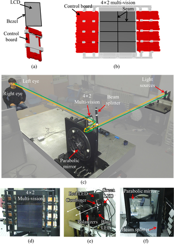
Table 1. System parameters.

Parameter	Value
Central wavelength of the light source (R, G, B)	(640, 525, 450 nm)
Resolution for an SLM (horizontal, vertical)	(1920, 1080)
Pixel pitch for an SLM (horizontal, vertical)	(57.7$\mu m$, 57.7$\mu m$)
Number of SLMs for multi-vision (horizontal, vertical)	(4, 2)
Resolution for multi-vision (horizontal, vertical)	(3840, 4320)
Size of the multi-vision	Diagonal 13.13 in.
Seam width of the multi-vision	3 mm
Size of the parabolic mirror	Diagonal 16 in.
F number of the parabolic mirror	4.5
Viewing distance	3.6 m
Size of viewing window (horizontal, vertical)	(28 mm, 28 mm)

Figure 2. Forward and inverse cascaded Fresnel transform model considering both eyes of the observer in a holographic multi-vision system.

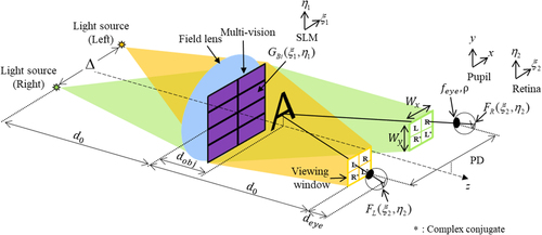
Figure 3. IPCT caused by (a) symmetric and (b) asymmetric pixel architectures in a binocular holographic multi-vision system, (c) diffraction pattern for the asymmetric pixel structure on the pupil plane, and (d) the intensity distribution of the diffraction pattern about the central axis of both eyes.

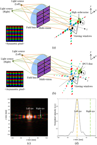
Figure 4. The numerical observation results from the full color multi-vision system with binocular parallax for the (a) reconstructed left 3D perspective image, (b) reconstructed right 3D perspective image, and experimental results for (c) a left 3D perspective image and (d) a right 3D perspective image.

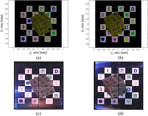
Figure 5. Numerical observation results for a reconstructed holographic image on the object plane (a)$d_{obj}=0m$, (b)$d_{obj}=0.5m$, (c)$d_{obj}=1.5m$, and (d)$d_{obj}=2.5m$ in the proposed multi-vision configuration.

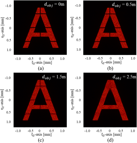
Figure 6. The relative luminance distribution of the reconstructed holographic image at the (a) horizontal intersection and (b) vertical intersection according to the distance to the object plane, and (c) the relationship between the uniformity and the distance to the object plane.

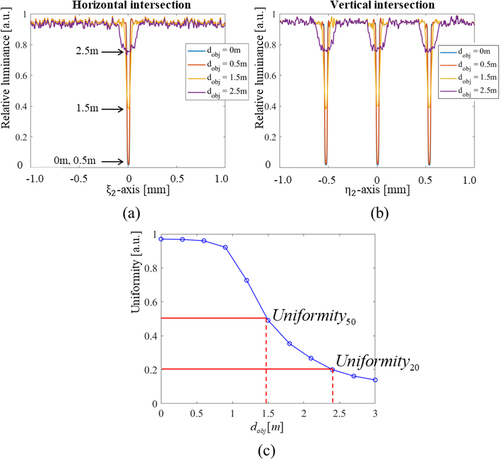
Figure 7. (a) Optical geometry for the circle of contribution determined by a point at the object plane and (b) minimum distance of seamless virtual reference plane corresponding to the viewing distance when the size of viewing window is 28 mm.

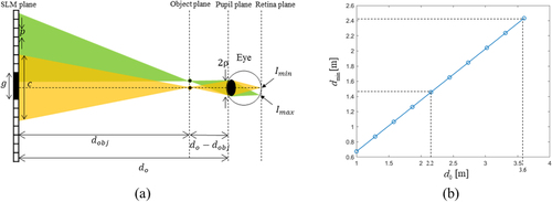
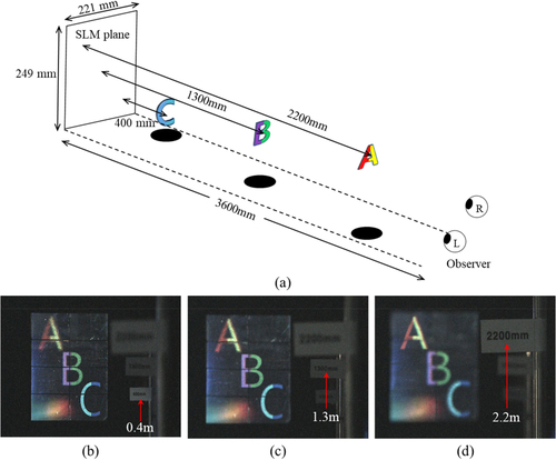
Figure 8. Experimental results of the 3D objects with difference depth: (a) Design values of the objects, and experimental results focused on (b) C at a distance of 0.4 m, (c) B at a distance of 1.3 m, and (d) A at a distance of 2.2 m from the SLM.