Figures & data
Fig 1. Time evolution of the nature run for the imperfect L96 model in the interval 0 ≤ t ≤. We choose four grid points which we depict in different colours.
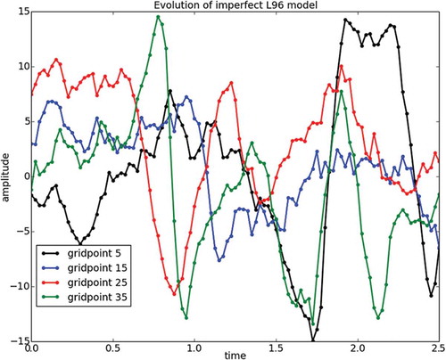
Fig 2. DA experiments in the L96 imperfect model with observations every time step and at every grid point. The left panel shows the true trajectory of variable x(2) (grey line), as well as the observations (grey dots). The coloured lines show the analysis trajectories by different DA methods (see legend). The middle panel shows the time evolution of the analysis RMSE. The right panel shows non-parametric statistics (25 percentile, median and 75 percentile) computed over time for each method.
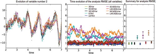
Fig 3. Land sea configuration used for our DA experiments. Twelve variables are observed and 12 are unobserved. We divide the grid into three types of variables: observed, unobserved and boundary variables.
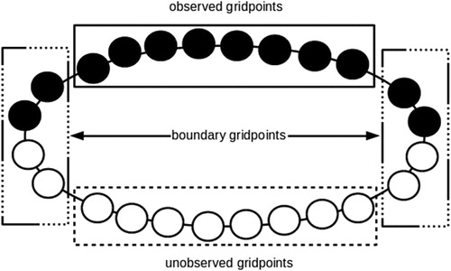
Fig 4. Analysis RMSE results for the imperfect L96 model under the land–sea configuration with observations every model step. We show the time evolution (left columns) and the summary statistics (right columns) for the different variables (rows). Different coloured lines correspond to different methods (see legend).
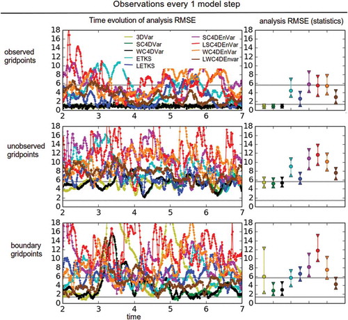
Fig 5. Same as Fig. 4, but with observations every two model steps.
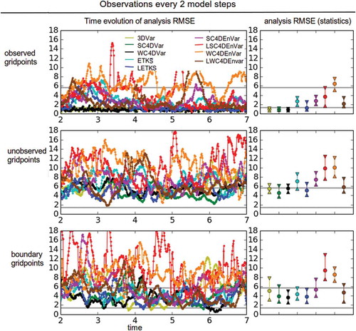
Fig 6. Median analysis RMSE over 1000 time steps for LETKS with the imperfect L96 with land–sea configuration and observations every two time steps. Different ensemble sizes (horizontal axis) and different localisation half-widths (vertical axis) are tested. Each panel represents a different kind of variable.
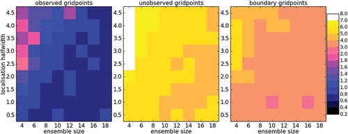
Fig 7. Median analysis RMSE over 1000 time steps for variational methods with the imperfect L96 with land–sea configuration and observations every two time steps. The top row shows results for SC4DEnVar, while the bottom row shows results for WC4DEnVar. Different numbers of observational times per analysis window (horizontal axis) and numbers of outer loops (vertical axis) are tested.
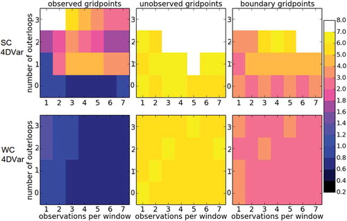
Fig 8. Median analysis RMSE over 1000 time steps non-localised EnVar methods (top row for SC4DEnVar, bottom row for WC4DEnVar) with the imperfect L96 with land–sea configuration and observations every two time steps. No outer loops (left half) and three outer loops (right half) are used. For each panel, we vary the ensemble size (horizontal axis) and the number of observations per window (vertical axis).
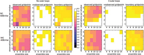
Fig 9. Median analysis RMSE over 1000 time steps EnVar methods (top rows for LSC4DEnVar, bottom rows for LWC4DEnVar) with the imperfect L96 with land–sea configuration and observations every two time steps. No outer loops (top half) and three outer loops (bottom half) are used. Different columns show different variables (left for observed, middle for unobserved and right for boundary variables). In each panel we show the variation with respect to three parameters: observations per window and localisation half-width in the horizontal axes, and ensemble size in the vertical axis.
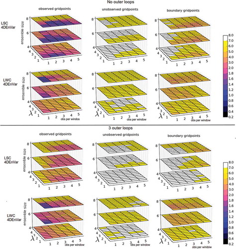
Fig 10. Hovmuller plots for the SWE model (with model error) showing the evolution of the truth. Each plot shows the time steps on the y-axis and the grid point number on the x-axis. The colour bars show the velocity, the height and the rain, respectively.
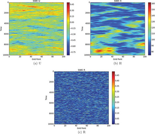
Fig 11. Climatological B matrix for the SWE model (with model error) over 100 grid points. See text for the description of its generation. Each panel shows the covariances between variables of the correspoding row and column in the figure.
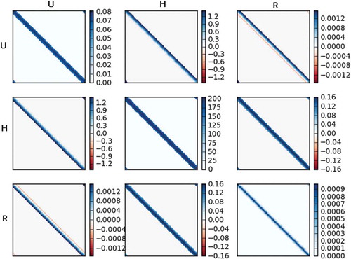
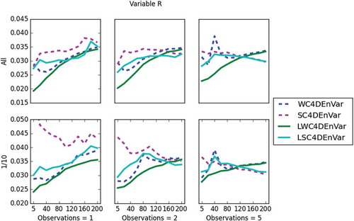
Fig 12. This plot shows the RMSE (y-axis) of all data assimilation methods for velocity, u, and the x-axis is the observation period. In the top three plots, all grid points are observed and in the bottom three plots only 1 in 10 grid points are observed. The two plots on the left show one observation per window, the middle two show two observations per window and the two on the right show five observations per window.
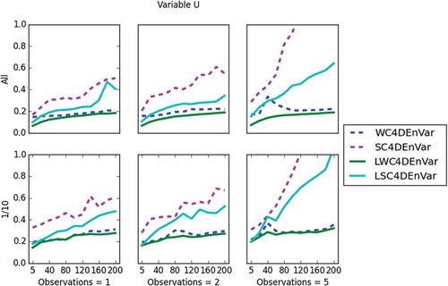
Fig 13. This plot shows the RMSE (y-axis) of all data assimilation methods for height, h, and the x-axis is the observation period. In the top three plots, all grid points are observed and in the bottom three plots only 1 in 10 grid points are observed. The two plots on the left show one observation per window, the middle two show two observations per window and the two on the right show five observations per window.
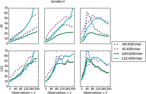
Fig 14. This plot shows the RMSE (y-axis) of all data assimilation methods for rain, r, and the x-axis is the observation period. In the top three plots, all grid points are observed and in the bottom three plots only 1 in 10 grid points are observed. The two plots on the left show one observation per window, the middle two show two observations per window and the two on the right show five observations per window.