Lake–atmosphere interactions at Alqueva reservoir: a case study in the summer of 2014

Figures & data

Fig. 1. Alqueva reservoir: geographic location, floating platforms and meteorological stations. A zoom from Alqueva-Montante platform equipped with the IRGASON instrument; details of the sonic anemometer, gas analyser and accelerometer.

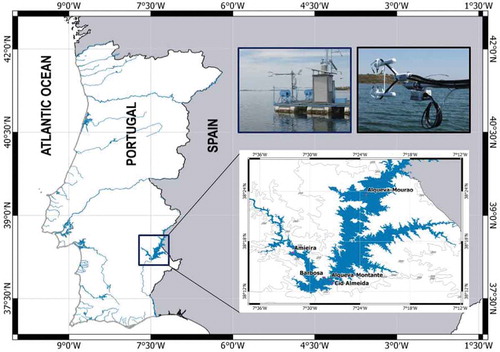
Fig. 2. Scheme of the apparatus developed for measurements of spectral underwater solar irradiance. Detail of the optical receiver and multilayer protecting frame of underwater device for measuring downwelling spectral irradiance.

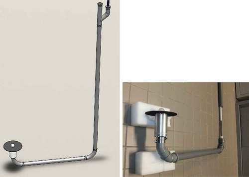
Fig. 3. Average normalized frequency-weighted co-spectra for CO₂, H₂O and sonic temperature (T_s) as a function of normalized frequency for the period 23–26 July 2014.

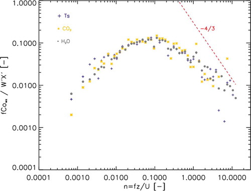
Fig. 4. (a) Footprint length (X₉₀) in the wind directions 270–90º; (b) scatterplot of footprint (X₉₀) and stability (z/L) during the period June–September 2014.

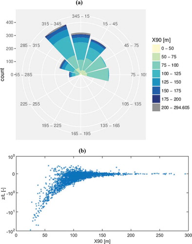
Fig. 5. Mean daily cycle of sensible heat flux (left y-axis; circles) and temperature difference between air (2 m) and near-surface water (right y-axis; stars) during the period June–September 2014.

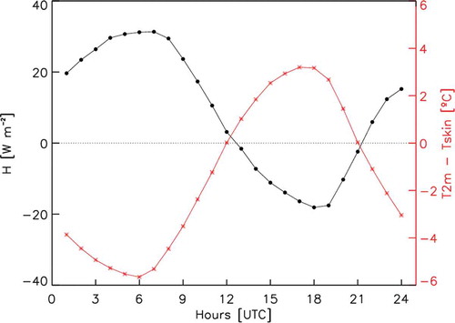
Fig. 6. (a) Mean daily cycle of latent heat flux (LE) (left y-axis; circles) and water vapour (right y-axis; stars); (b) mean daily cycle of latent heat flux (left y-axis; circles) and wind speed (right y-axis; stars), during the period June–September 2014.

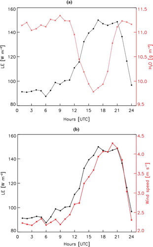
Fig. 7. (a) Mean daily cycle of net radiation (Rn), water column heat storage (∆Q), latent heat flux (LE) and sensible heat flux (H) during the period June–September 2014. (b) Average energy residual (Res) measured with different depths for water column heat storage (∆Q) calculations during the period June–September 2014. EBC = energy balance closure.

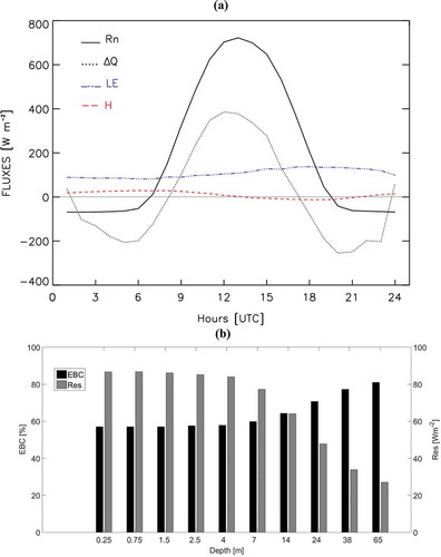
Fig. 8. Mean daily cycle of CO₂ flux (left y-axis; circles) and CO₂ concentration (right y-axis; stars) during the period June–September 2014.

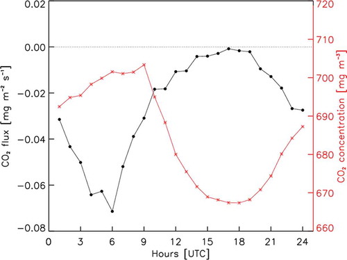
Fig. 9. Profiles in Alqueva-Montante on 10 July 2014: (a) underwater downwelling spectral irradiance measured with the new devices; (b) underwater downwelling spectral radiance with the device from Potes et al. (2013). Profiles are given in digital numbers (DN); output values without calibration.

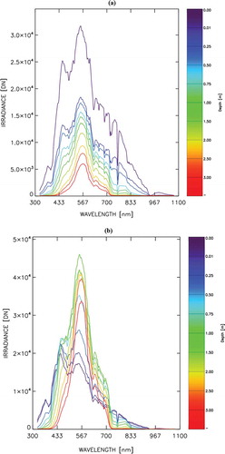
Table 1. Measurement details

Date	Time (UTC)	Measurement location	PAR attenuation coefficient^a (m^−1)
Smith and Baker (1981)	–	Pure water	0.166
10 July 2014	10:24	Alqueva-Montante	0.709 ± 0.006
14 July 2014	10:32	Swimming complex	0.191 ± 0.002
30 July 2014	11:19	Alqueva-Montante	0.849 ± 0.025
27 August 2014	10:25	Alqueva-Montante	0.875 ± 0.023
27 August 2014	14:30	Alqueva-Mourão	1.112 ± 0.019
25 September 2014	15:31	Alqueva-Montante	1.055 ± 0.004
25 September 2014	10:39	Alqueva-Mourão	1.459 ± 0.007

^aPhotosynthetically active radiation attenuation coefficient for the layer 0–3 m.

Fig. 10. Profiles of underwater downwelling spectral irradiance: (a) in the municipal swimming complex of Évora; (b) in Alqueva reservoir. Profiles are in percentage of surface irradiance.

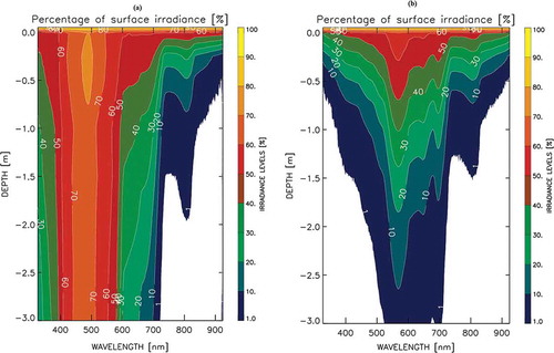
Fig. 11. Spectral attenuation coefficient for the field campaigns described in Table 1.

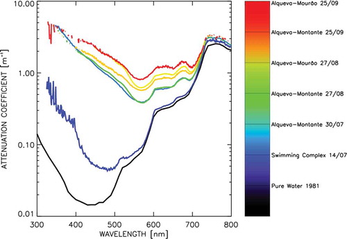
Fig. 12. Wind rose for 23 selected days in the period 13–15 UTC (units of m s⁻¹) for (a) Barbosa and (b) Cid Almeida stations (1 min resolution). The criteria for the selection were: daily maximum of the temperature difference between air (in Barbosa station) and water (in Alqueva-Montante) greater than 7 ºC, and daily average wind speed lower than 3.5 m s⁻¹ at Barbosa station.

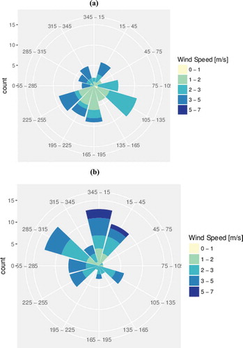
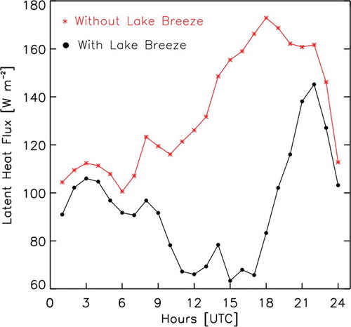
Fig. 13. Mean daily cycle of latent heat flux for 23 selected days with development of lake breeze and 27 selected days without lake breeze.

Potes, M., Costa, M. J., Salgado, R., Bortoli, D., Serafim, A. and co-authors 2013. Spectral measurements of underwater downwelling radiance of inland water bodies. Tellus-A 65, 20774. DOI:10.3402/tellusa.v65i0.20774.

 Web of Science ®Google Scholar

Smith, R. C. and Baker, K. S. 1981. Optical properties of the clearest natural waters (200-800 nm). Appl. Opt. 20, 177–184.

 PubMed Web of Science ®Google Scholar