Figures & data
Figure 1. The boundary layer structure in the linear model.
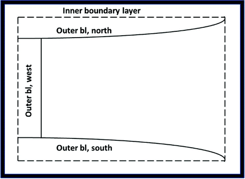
Figure 2. Horizontal velocity at the surface in the linear model (left) and MITgcm (right). The arrows indicate the direction and the colors indicate the strength of the flow.
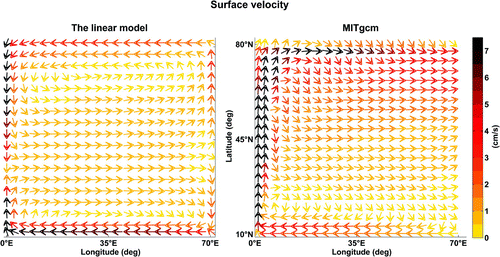
Figure 3. Mid-basin transects of the zonal velocity at E in the linear model (left) and in MITgcm (right).
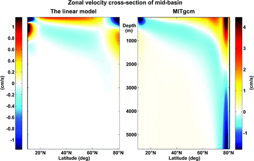
Figure 4. Cross-sections of the meridional velocity at N (lower row) and
N (upper row) for the linear model (left column) and MITgcm (right column).
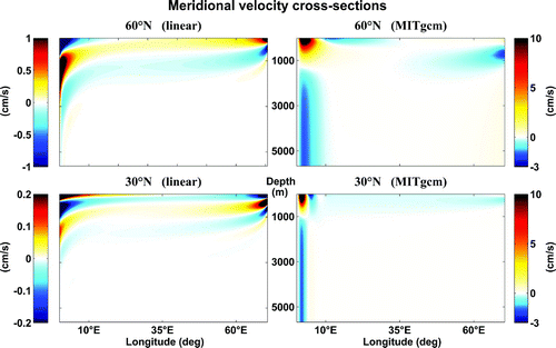
Figure 5. Depth-integrated vertical velocity for the linear model (left) and MITgcm (right). In the north and south, only the vertical velocities associated with vertical mixing are shown, as only these contribute to the area-averaged w. The wave-like disturbances in the north in the MITgcm simulation are linked to convection (rather than numerical instability).
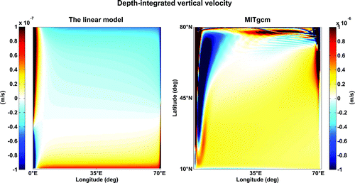
Figure 6. Zonally averaged potential temperature (top) and convective adjustment index (bottom). In areas where the index is greater than zero, the vertical diffusivity is large due to enhanced mixing.
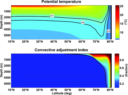
Figure 7. A schematic illustrating the differences in the surface flow between the linear and nonlinear models.
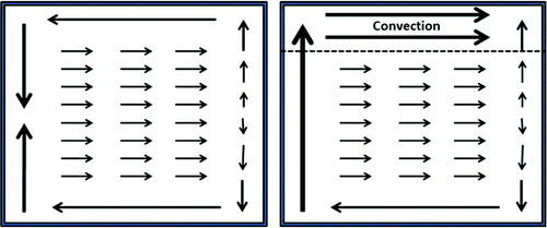
Figure 8. Left: A vertical profile of the mean zonal velocity in the convective region in MITgcm (blue line) and calculated according to Equation (Equation18(18) ) (yellow line). Right: The mean stratification in convective region (blue line) and just south of the convective region (yellow line) in MITgcm.
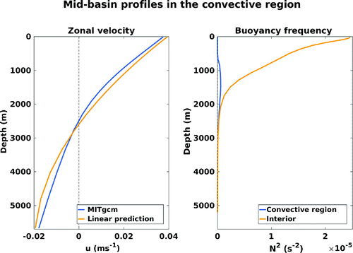
Figure 9. Horizontal (blue arrows and numbers) and vertical (boxes - red numbers indicate upwelling while blue numbers indicate downwelling) transports for the upper 1200 m in MITgcm. All transports are given in Sv.
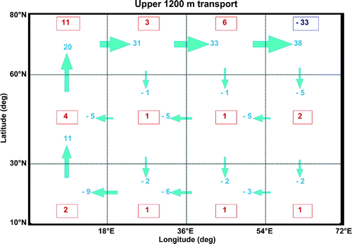
Figure 10. The meridional overturning streamfunction, , for the (top) linear model and (bottom) MITgcm. Positive
indicates clockwise rotation. Top figure: The linear model exhibits two overturning cells confined to the southern and northern part of the basin. Bottom figure: MITgcm exhibits one positive overturning cell spanning the basin and one narrow, negative cell in the north. The latter is a consequence of the no-slip condition at the northern wall.
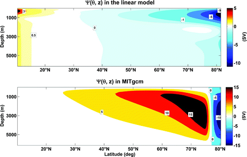
Figure 11. Maximum overturning (dark blue), northern boundary layer width (light blue), north-east downwelling (red), meridional heat transport at N (brown) and heat transport in the southern boundary layer (green) sensitivity to vertical mixing,
. The maximum overturning include three values from Winton (1996), scaled by 0.7.
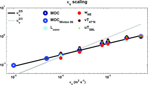
Figure 12. Terms in the buoyancy equation in the western boundary region, at N and 300 m depth from MITgcm.
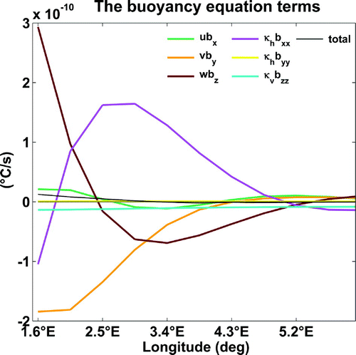
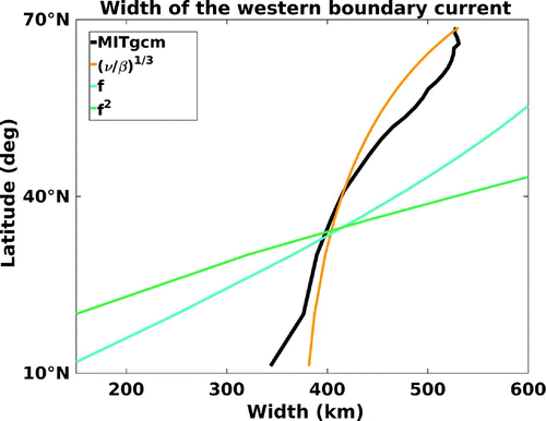
Figure 13. Scaling of the width of the western boundary current (black line) vs. Munk layer (orange line), the Coriolis frequency f (blue line) and (dark green line).