1,747
Views
23
CrossRef citations to date
0
Altmetric
Research Article

Multi-decadal variations of the South Indian Ocean subsurface temperature influenced by Pacific Decadal Oscillation

, , , &
Article: 1308055 | Received 23 Jan 2017, Accepted 14 Mar 2017, Published online: 11 Apr 2017

Figures & data

Fig. 1. Time series of PDO index. The red and blue bars stand for the model CTRL experiment and the green curve represents the ERSST reanalysis.
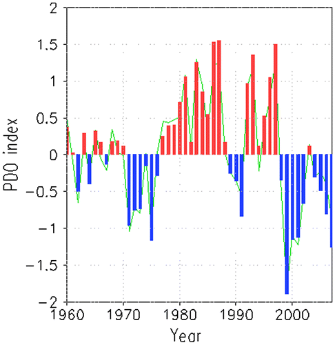
Fig. 1. Time series of PDO index. The red and blue bars stand for the model CTRL experiment and the green curve represents the ERSST reanalysis.

Fig. 2. Linear trends (°C/century) of zonal-mean temperature in the Indian Ocean during the periods 1960–98, 1960–76 (Period I) and 1977–98 (Period II) from SODA reanalysis.
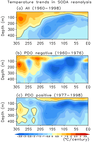
Fig. 2. Linear trends (°C/century) of zonal-mean temperature in the Indian Ocean during the periods 1960–98, 1960–76 (Period I) and 1977–98 (Period II) from SODA reanalysis.

Fig. 3. Left panels: linear trends (°C/century) of zonal-mean temperature in the Indian Ocean during the period 1960–98 in different model experiments for (a) CTRL, (b) IND and (c) DIF. Middle panels and right panels are the same as the left panels but for the periods 1960–76 and 1977–98, respectively. The box in (a) indicates the domain of 9–15°S and 100–300 m depth.
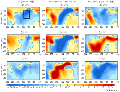
Fig. 3. Left panels: linear trends (°C/century) of zonal-mean temperature in the Indian Ocean during the period 1960–98 in different model experiments for (a) CTRL, (b) IND and (c) DIF. Middle panels and right panels are the same as the left panels but for the periods 1960–76 and 1977–98, respectively. The box in (a) indicates the domain of 9–15°S and 100–300 m depth.

Fig. 4. Time series of temperature anomaly (°C) averaged over the domain of 9°–15°S, 30°–130°E between 100 and 300 m (a box in Fig. 3a) for SODA (black), CTRL (red), IND (green) and DIF (blue). The dashed lines denote the linear trends of the corresponding same colour curves for the distinct periods 1960–76 (Period I) and 1977–98 (Period II).
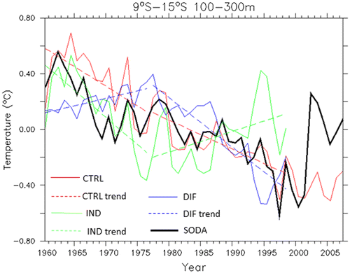
Fig. 4. Time series of temperature anomaly (°C) averaged over the domain of 9°–15°S, 30°–130°E between 100 and 300 m (a box in Fig. 3a) for SODA (black), CTRL (red), IND (green) and DIF (blue). The dashed lines denote the linear trends of the corresponding same colour curves for the distinct periods 1960–76 (Period I) and 1977–98 (Period II).

Fig. 5. The tropical Pacific (averaged over 5°S–5°N, 120°E–70°W, blue curve) and the SIO (averaged over 9°S–15°S, 30°E–130°E, green curve) trade wind stress anomalies (10−3 N/m2). The dashed lines indicate the linear trend for the periods 1960–76 and 1977–98.
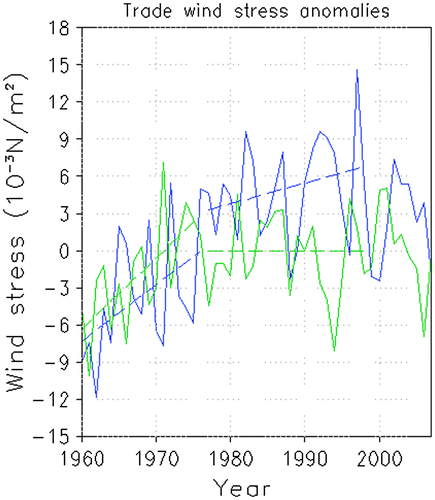
Fig. 5. The tropical Pacific (averaged over 5°S–5°N, 120°E–70°W, blue curve) and the SIO (averaged over 9°S–15°S, 30°E–130°E, green curve) trade wind stress anomalies (10−3 N/m2). The dashed lines indicate the linear trend for the periods 1960–76 and 1977–98.

Fig. 6. Time series of ITF volume transport (Sv) (a) and ITF heat transport (PW) (b). The dashed line stands for the linear trends for the periods 1960–76 and 1977–98.
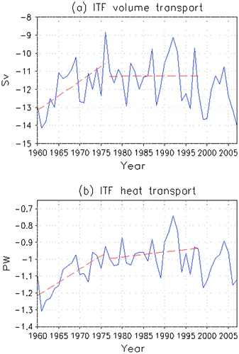
Fig. 6. Time series of ITF volume transport (Sv) (a) and ITF heat transport (PW) (b). The dashed line stands for the linear trends for the periods 1960–76 and 1977–98.

Fig. 7. Time-evolving annual mean temperature anomalies averaged between 9–15°S and 100–300 m in the IO: (a) for CTRL and (c) for IND and averaged between 10°S–10°N in the Pacific at the same depth from 1960 to 2007: (b) for CTRL and (d) for IND.
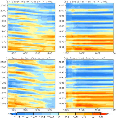
Fig. 7. Time-evolving annual mean temperature anomalies averaged between 9–15°S and 100–300 m in the IO: (a) for CTRL and (c) for IND and averaged between 10°S–10°N in the Pacific at the same depth from 1960 to 2007: (b) for CTRL and (d) for IND.

Fig. 8. (a) The climatological annual mean Ekman pumping velocity (EPV) from interannual CORE-II forcing (1 × 10−6 m/s, upwelling is red and downwelling is blue). (b) and (c) are the EPV linear trends (1 × 10−7 m/s year−1) for the periods 1960–76 and 1977–98, respectively.
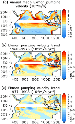
Fig. 8. (a) The climatological annual mean Ekman pumping velocity (EPV) from interannual CORE-II forcing (1 × 10−6 m/s, upwelling is red and downwelling is blue). (b) and (c) are the EPV linear trends (1 × 10−7 m/s year−1) for the periods 1960–76 and 1977–98, respectively.

Fig. 9. (a) Regression between PDO index and zonal wind stress anomaly (10−3 N/m2 sd−1) during the period 1960–98 (colour shading) and climatological annual mean wind stress (N/m2) (arrows). (b) Regression between PDO index and ocean temperature anomaly averaged over 10°S–10°N along the equator (°C sd−1).
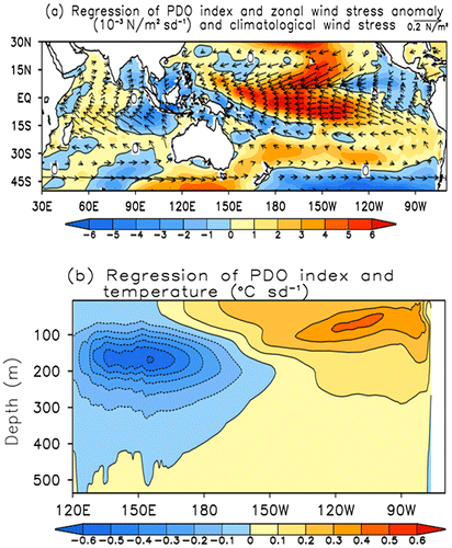
Fig. 9. (a) Regression between PDO index and zonal wind stress anomaly (10−3 N/m2 sd−1) during the period 1960–98 (colour shading) and climatological annual mean wind stress (N/m2) (arrows). (b) Regression between PDO index and ocean temperature anomaly averaged over 10°S–10°N along the equator (°C sd−1).

Fig. 10. The linear trends of temperature anomaly (°C/decade) along the equatorial Pacific during the periods 1960–98 (a), 1960–76 (b) and 1977–98 (c) in CTRL. (d) Time series of temperature anomaly index (averaged over 10°S–10°N, 120°E–160°E between 100 and 300 m) and its linear trends during the periods 1960–76 and 1977–98 in CTRL.
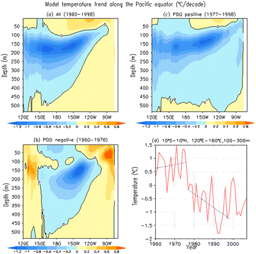
Fig. 10. The linear trends of temperature anomaly (°C/decade) along the equatorial Pacific during the periods 1960–98 (a), 1960–76 (b) and 1977–98 (c) in CTRL. (d) Time series of temperature anomaly index (averaged over 10°S–10°N, 120°E–160°E between 100 and 300 m) and its linear trends during the periods 1960–76 and 1977–98 in CTRL.