985
Views
7
CrossRef citations to date
0
Altmetric
Research Article

High-resolution data assimilation through stochastic subgrid tensor and parameter estimation from 4DEnVar

&
Article: 1308772 | Received 30 Jan 2017, Accepted 13 Mar 2017, Published online: 07 Apr 2017

Figures & data

Figure 1. RMSE comparison in terms of free surface height (a) and velocity (b) between various configurations. PO: Perturbed observation. LC: Localized covariance approach. Standard model: no subgrid tensor parameterization. N: number of ensemble member.
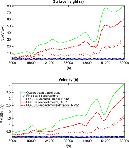
Figure 1. RMSE comparison in terms of free surface height (a) and velocity (b) between various configurations. PO: Perturbed observation. LC: Localized covariance approach. Standard model: no subgrid tensor parameterization. N: number of ensemble member.

Figure 2. RMSE comparison in terms of free surface height (a) and velocity (b) between various configurations of 4DEnVar. PO: Perturbed observation. LC: Localized covariance approach. Standard model: no subgrid tensor parameterization. N: number of ensemble member. 6 DA cycle phase:  s. Forecast phase:  s.
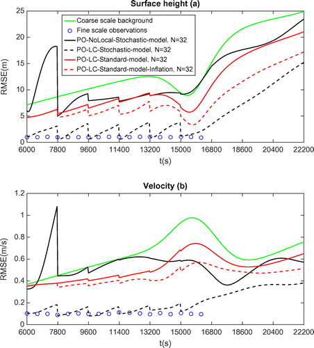
Figure 2. RMSE comparison in terms of free surface height (a) and velocity (b) between various configurations of 4DEnVar. PO: Perturbed observation. LC: Localized covariance approach. Standard model: no subgrid tensor parameterization. N: number of ensemble member. 6 DA cycle phase:  s. Forecast phase:  s.

Figure 3. Ensemble spread in terms of free surface height (a) and velocity (b): standard model (circle) with ensemble in function of initial states; standard model (triangle) with ensemble in function of initial states but with multiplicative inflation technique; subgrid model (square) with ensemble in function of initial parameters.
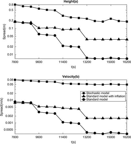
Figure 3. Ensemble spread in terms of free surface height (a) and velocity (b): standard model (circle) with ensemble in function of initial states; standard model (triangle) with ensemble in function of initial states but with multiplicative inflation technique; subgrid model (square) with ensemble in function of initial parameters.

Figure 4. RMSE comparison in terms of free surface height (a) and velocity (b) between various subgrid model configurations in Table of stochastic shallow water model (17). The meaning of different is shown in Table .
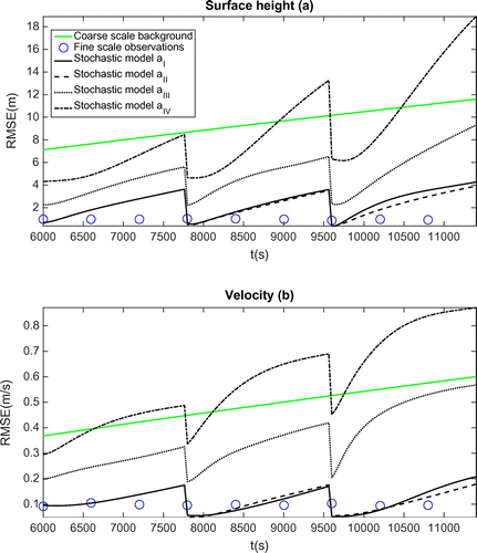
Figure 4. RMSE comparison in terms of free surface height (a) and velocity (b) between various subgrid model configurations in Table 1 of stochastic shallow water model (17). The meaning of different is shown in Table 1.

Figure 5. The RMSE of height comparison in the 1st and 2nd cycle as a function of Cut-off distance (LC, localized covariance) or local domain size (LA, local analysis).
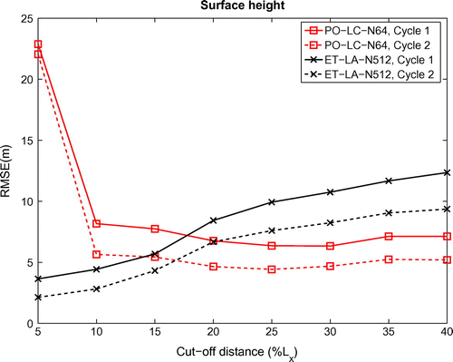
Figure 5. The RMSE of height comparison in the 1st and 2nd cycle as a function of Cut-off distance (LC, localized covariance) or local domain size (LA, local analysis).

Figure 6. RMSE comparison in terms of free surface height (a) and lengthwise velocity (b) between various configurations of 4DEnVar. ET, ensemble transform. PO, perturbed observation. DE, deterministic ensemble. LC, localized covariance. LA, local analysis. ET-LA-N128-Stochastic (solid line) case with shows ensemble ‘blow up’; ET-LA-N128-Stochastic (dashed line) with shows ensemble collapse; ET-LA-N512-Stochastic (dotted line) used ensemble relaxation inflation technique for state ensemble; PO-LC-N64-Standard used standard model and multiplicative inflation technique for state ensemble.
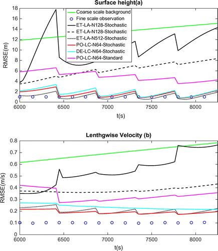
Figure 6. RMSE comparison in terms of free surface height (a) and lengthwise velocity (b) between various configurations of 4DEnVar. ET, ensemble transform. PO, perturbed observation. DE, deterministic ensemble. LC, localized covariance. LA, local analysis. ET-LA-N128-Stochastic (solid line) case with shows ensemble ‘blow up’; ET-LA-N128-Stochastic (dashed line) with shows ensemble collapse; ET-LA-N512-Stochastic (dotted line) used ensemble relaxation inflation technique for state ensemble; PO-LC-N64-Standard used standard model and multiplicative inflation technique for state ensemble.

Figure 7. Power spectral density of ensemble anomalies for the forecast ensemble (a), the analysis ensemble by LC (b) and LA (c).
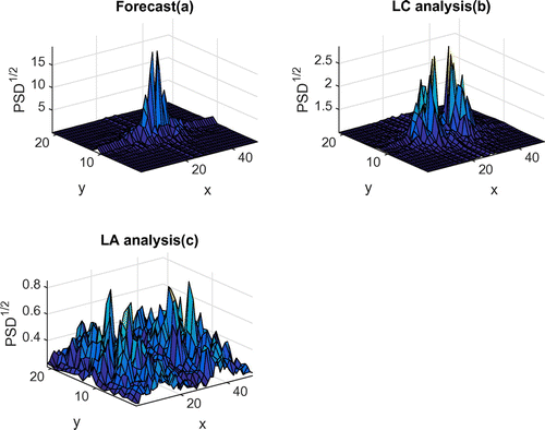
Figure 7. Power spectral density of ensemble anomalies for the forecast ensemble (a), the analysis ensemble by LC (b) and LA (c).

Figure 8. Comparison of various configurations of 4DEnVar w.r.t. (a) Mean surface height of the wave crest region as a function of time and (b) The RMSE against observation at observation time. 4DVar, 4DEnVar-PO-LC and 4DEnVar-ET-LA are tested with the standard model; 4DEnVar-PO-LC-Sto and 4DEnVar-ET-LA-Sto are tested with the stochastic model. LC, localized covariance. PO, perturbed observation. LA, local analysis. ET, ensemble transformation.
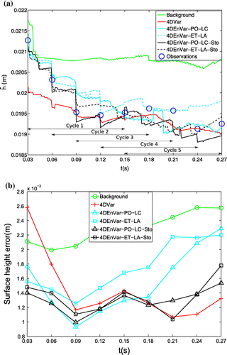
Figure 8. Comparison of various configurations of 4DEnVar w.r.t. (a) Mean surface height of the wave crest region as a function of time and (b) The RMSE against observation at observation time. 4DVar, 4DEnVar-PO-LC and 4DEnVar-ET-LA are tested with the standard model; 4DEnVar-PO-LC-Sto and 4DEnVar-ET-LA-Sto are tested with the stochastic model. LC, localized covariance. PO, perturbed observation. LA, local analysis. ET, ensemble transformation.

Figure 9. Ensemble Spread in terms of free surface height (a) and lengthwise velocity (b) for: standard model cycle 1 and cycle 5 (circle with solid/dashed line); stochastic model cycle 1 and cycle 5 (square with solid/dashed line).
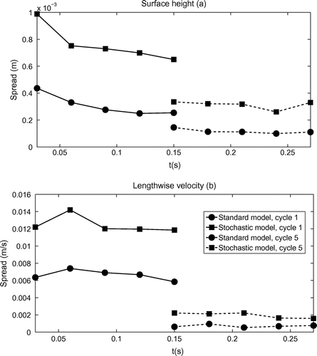
Figure 9. Ensemble Spread in terms of free surface height (a) and lengthwise velocity (b) for: standard model cycle 1 and cycle 5 (circle with solid/dashed line); stochastic model cycle 1 and cycle 5 (square with solid/dashed line).

Table 1. Different combination of the terms composing the subgrid model.