2,017
Views
7
CrossRef citations to date
0
Altmetric
Articles

Relative strength of the Antarctic Circumpolar Current and Atlantic Meridional Overturning Circulation

&
Article: 1338884 | Received 22 Dec 2016, Accepted 29 May 2017, Published online: 26 Jun 2017

Figures & data

Figure 1. Schematic of the two layer model of Gnanadesikan (Citation1999) for the depth, h, of the global pycnocline. , , and are the water mass transformations between the two layers associated with northward Ekman transport in the Southern Ocean, Southern Ocean eddies, diapycnal mixing in the ocean interior, and North Atlantic Deep Water formation, respectively.
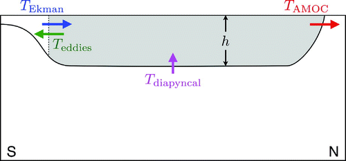
Figure 1. Schematic of the two layer model of Gnanadesikan (Citation1999) for the depth, h, of the global pycnocline. , , and are the water mass transformations between the two layers associated with northward Ekman transport in the Southern Ocean, Southern Ocean eddies, diapycnal mixing in the ocean interior, and North Atlantic Deep Water formation, respectively.

Figure 2. Neutral density sections from WOCE in the Atlantic sector, adapted with permission from the WOCE Atlantic Ocean Atlas (Koltermann et al., Citation2011). The coloured bars at the bottom of each section correspond to the coloured lines on the map (upper right panel). The lower section is a composite between the A23 and A16 sections.
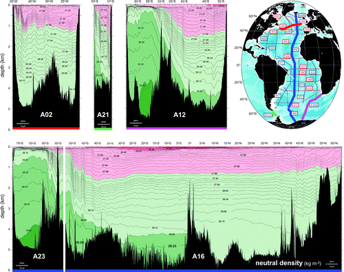
Figure 2. Neutral density sections from WOCE in the Atlantic sector, adapted with permission from the WOCE Atlantic Ocean Atlas (Koltermann et al., Citation2011). The coloured bars at the bottom of each section correspond to the coloured lines on the map (upper right panel). The lower section is a composite between the A23 and A16 sections.

Figure 3. Neutral density at (a) and (b) , reproduced with permission from the WOCE Atlantic Atlas (Koltermann et al., Citation2011).
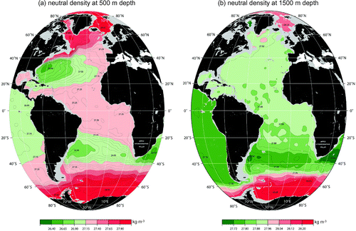
Figure 3. Neutral density at (a) and (b) , reproduced with permission from the WOCE Atlantic Atlas (Koltermann et al., Citation2011).

Figure 4. (a) Schematic diagram showing the key elements of the thermal wind model. The solid black lines indicate the neutral density surfaces which are flat along the eastern boundary of the Atlantic but slope and can outcrop in the sections across the Southern Ocean and North Atlantic. The dashed lines represent the sloping boundaries to the north and south of the Southern Ocean section, and to the east and west of the North Atlantic section. The three depth scales , and are also indicated – see main text for details. The long solid purple arrows symbolise the ACC, and the long solid red and blue arrows symbolise the upper and lower limbs of the AMOC. (b) Schematic of the model across the North Atlantic section. The strength of the AMOC is set by integrating the thermal wind relation between the sloping eastern (dashed red) and western (dashed blue) boundaries, from the assumed level of no motion at to the surface . (c) Schematic of the model across the Southern Ocean section. The strength of the ACC is set by integrating the thermal wind relation between the sloping northern (dashed red) and southern (dashed blue) boundaries, from to the surface .
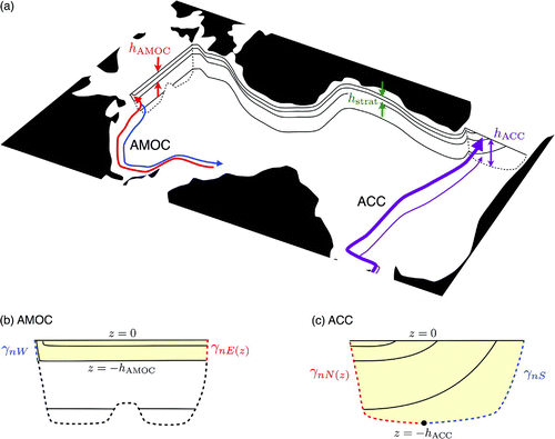
Figure 4. (a) Schematic diagram showing the key elements of the thermal wind model. The solid black lines indicate the neutral density surfaces which are flat along the eastern boundary of the Atlantic but slope and can outcrop in the sections across the Southern Ocean and North Atlantic. The dashed lines represent the sloping boundaries to the north and south of the Southern Ocean section, and to the east and west of the North Atlantic section. The three depth scales , and are also indicated – see main text for details. The long solid purple arrows symbolise the ACC, and the long solid red and blue arrows symbolise the upper and lower limbs of the AMOC. (b) Schematic of the model across the North Atlantic section. The strength of the AMOC is set by integrating the thermal wind relation between the sloping eastern (dashed red) and western (dashed blue) boundaries, from the assumed level of no motion at to the surface . (c) Schematic of the model across the Southern Ocean section. The strength of the ACC is set by integrating the thermal wind relation between the sloping northern (dashed red) and southern (dashed blue) boundaries, from to the surface .

Figure 5. The (a) e-folding depth, (b) surface neutral density and (c) asymptotic abyssal neutral density, obtained by fitting the exponential neutral density profile (Equation3) to the WOCE climatological data of Gouretski and Koltermann (Citation2004).

Figure 5. The (a) e-folding depth, (b) surface neutral density and (c) asymptotic abyssal neutral density, obtained by fitting the exponential neutral density profile (Equation3(3) ) to the WOCE climatological data of Gouretski and Koltermann (Citation2004).
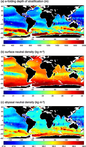
Figure 6. Neutral density profiles along the sloping western () and eastern () boundaries at N in the Atlantic (solid blue and red lines), along the sloping southern () and northern () boundaries at E in the Southern Ocean (dashed blue and red lines), and the fitted exponential profile with (solid black line).
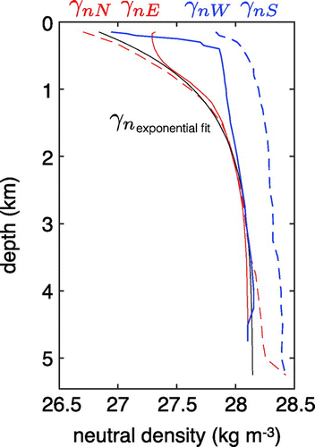
Figure 6. Neutral density profiles along the sloping western () and eastern () boundaries at N in the Atlantic (solid blue and red lines), along the sloping southern () and northern () boundaries at E in the Southern Ocean (dashed blue and red lines), and the fitted exponential profile with (solid black line).

Figure 7. AMOC streamfunction profiles (Sv) at 26.5N for the periods April 2004 to March 2008 and April 2008 to March 2012. Reproduced with permission from Smeed et al. (Citation2014) under the Creative Commons Attribution 3.0 License.
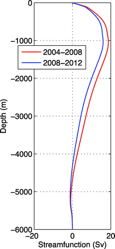
Figure 7. AMOC streamfunction profiles (Sv) at 26.5N for the periods April 2004 to March 2008 and April 2008 to March 2012. Reproduced with permission from Smeed et al. (Citation2014) under the Creative Commons Attribution 3.0 License.

Figure 8. Contours of as a function of the two depth-scale ratios, and . The blue shading indicates the observation-based estimates of the depth-scale ratios, from which we infer , consistent with the observed value of .
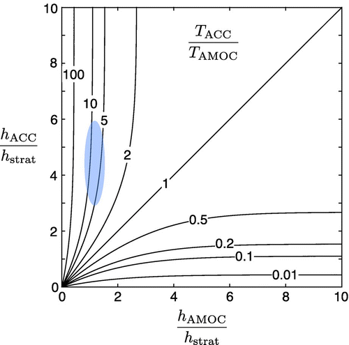
Figure 8. Contours of as a function of the two depth-scale ratios, and . The blue shading indicates the observation-based estimates of the depth-scale ratios, from which we infer , consistent with the observed value of .