8,782
Views
30
CrossRef citations to date
0
Altmetric
Articles

A short review of numerical cloud-resolving models

&
Article: 1373578 | Received 10 Jan 2017, Accepted 02 Aug 2017, Published online: 19 Sep 2017

Figures & data

Fig. 1. (a) Schematic of a population of clouds over a tropical ocean; thin (thick) arrows represent convective (stratiform) updraught and downdraught, while heavy convective (lighter stratiform) rain is indicated by narrow (wider) hatchings – adapted from Houze et al. (Citation1980), ©Copyright 1980 American Meteorological Society (AMS), see also Houze and Betts (Citation1981). (b) Three-dimensional view of a cloud field simulated by a CRM – adapted from Guichard (Citation1995), see also Guichard et al. (Citation1997).
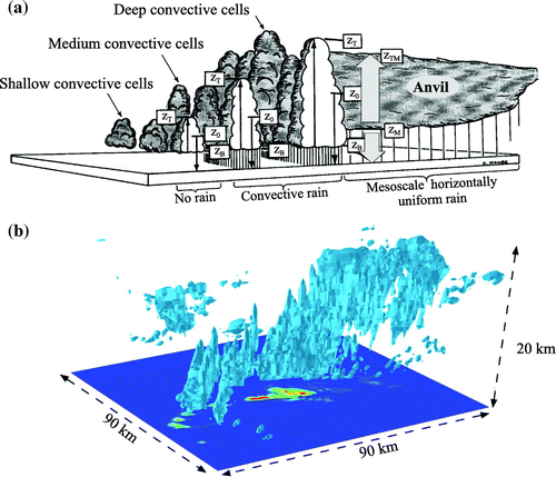
Fig. 1. (a) Schematic of a population of clouds over a tropical ocean; thin (thick) arrows represent convective (stratiform) updraught and downdraught, while heavy convective (lighter stratiform) rain is indicated by narrow (wider) hatchings – adapted from Houze et al. (Citation1980), ©Copyright 1980 American Meteorological Society (AMS), see also Houze and Betts (Citation1981). (b) Three-dimensional view of a cloud field simulated by a CRM – adapted from Guichard (Citation1995), see also Guichard et al. (Citation1997).

Fig. 2. Vertical structure of the convective processes operating in the budget of temperature (a) and water vapour (b) within an atmosphere experiencing deep convection over a tropical ocean. The solid black lines corresponds to the apparent heat source and moisture sink (Q1, Q2) that are parametrized in large-scale models; the red dotted, blue dashed and orange dashed-dotted lines indicate, respectively the total latent heat release due to microphysical processes (Q*, Q), the impact of turbulent and convective transport, and divergence of radiative fluxes (Qrad). (Results from a CRM simulation presented in Guichard et al. (Citation2000), the slots show seven-day mean profiles over an area 256 km wide.)
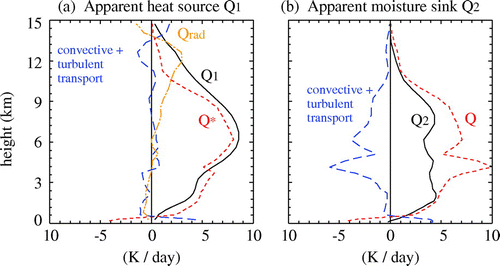
Fig. 2. Vertical structure of the convective processes operating in the budget of temperature (a) and water vapour (b) within an atmosphere experiencing deep convection over a tropical ocean. The solid black lines corresponds to the apparent heat source and moisture sink (Q1, Q2) that are parametrized in large-scale models; the red dotted, blue dashed and orange dashed-dotted lines indicate, respectively the total latent heat release due to microphysical processes (Q*, Q), the impact of turbulent and convective transport, and divergence of radiative fluxes (Qrad). (Results from a CRM simulation presented in Guichard et al. (Citation2000), the slots show seven-day mean profiles over an area 256 km wide.)

Fig. 3. Illustration of one of the first LES of shallow cumulus clouds: (a) 3D view of the cumulus simulation after 4 h of simulation. The domain is a 2 × 2 × 2 km3 cube and the grid size is 50 m in all three directions, (b) horizontal cross-sections at 775 m of the vertical velocity (w), potential temperature (θ), specific humidity (qv) and liquid mixing ratio (ql), with interval between isolines of, respectively, 0.61 m s−1, 0.92 K, 0.42 g kg−1 and 0.091 g kg−1 – these cross-sections highlight the strong correlations among those variables – adapted from Sommeria (Citation1976), ©Copyright 1976 AMS.
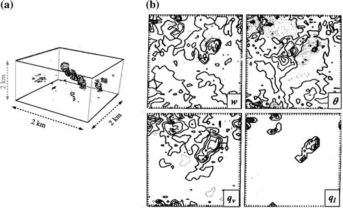
Fig. 3. Illustration of one of the first LES of shallow cumulus clouds: (a) 3D view of the cumulus simulation after 4 h of simulation. The domain is a 2 × 2 × 2 km3 cube and the grid size is 50 m in all three directions, (b) horizontal cross-sections at 775 m of the vertical velocity (w), potential temperature (θ), specific humidity (qv) and liquid mixing ratio (ql), with interval between isolines of, respectively, 0.61 m s−1, 0.92 K, 0.42 g kg−1 and 0.091 g kg−1 – these cross-sections highlight the strong correlations among those variables – adapted from Sommeria (Citation1976), ©Copyright 1976 AMS.

Fig. 4. Schematic of expected differences in surface winds between a 3D (a) and a 2D (b) simulation. The arrows indicate the surface winds resulting from downdraught spreading at the surface as a cold pool, with thicker arrows representing higher velocities – adapted from Tompkins (Citation2000), © Copyright 2000 AMS.
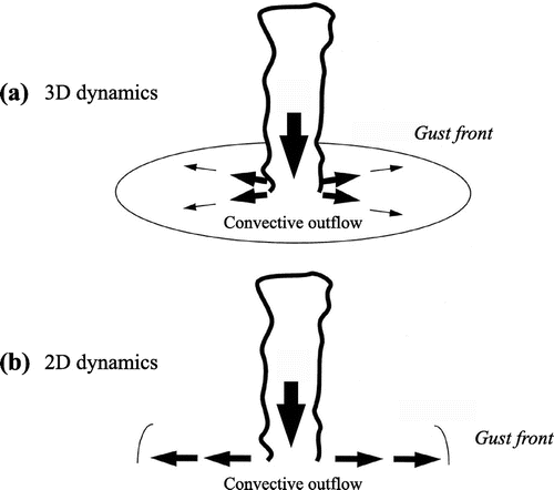
Fig. 4. Schematic of expected differences in surface winds between a 3D (a) and a 2D (b) simulation. The arrows indicate the surface winds resulting from downdraught spreading at the surface as a cold pool, with thicker arrows representing higher velocities – adapted from Tompkins (Citation2000), © Copyright 2000 AMS.

Fig. 5. Horizontal-mean vertical cross-sections of vertical velocity (contour interval 1 m s−1) and rain water mixing ratio (shaded) of squall-line simulations using grid spacing of (a) 1000 m, (b) 500 m, (c) 250 m and (d) 125 m in all three directions, except for (a) where the grid spacing is 500 m on the vertical – adapted from Bryan et al. (Citation2003), ©Copyright 2003 AMS.
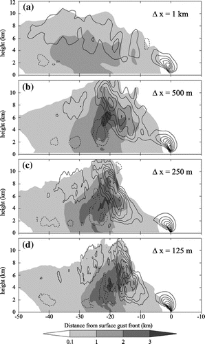
Fig. 5. Horizontal-mean vertical cross-sections of vertical velocity (contour interval 1 m s−1) and rain water mixing ratio (shaded) of squall-line simulations using grid spacing of (a) 1000 m, (b) 500 m, (c) 250 m and (d) 125 m in all three directions, except for (a) where the grid spacing is 500 m on the vertical – adapted from Bryan et al. (Citation2003), ©Copyright 2003 AMS.

Fig. 6. Relative contributions of the resolved (warm colours) and subgrid (cold colours) motions to the total turbulent kinetic energy (TKE) within various convective boundary layers simulated by LES as a function of the dimensionless mesh Δx/(h + hc) where Δx is the LES grid size and h + hc is the height of the cloudy boundary layer. The grey box-and-whiskers plots show the median and the variance of the resolved TKE per class of Δx/(h + hc) – adapted from Honnert et al. (Citation2011), ©Copyright 2011 AMS.
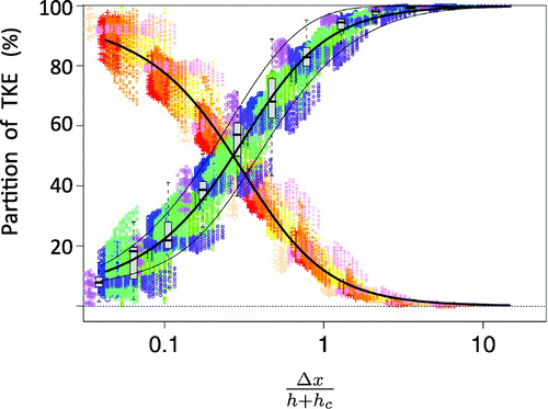
Fig. 6. Relative contributions of the resolved (warm colours) and subgrid (cold colours) motions to the total turbulent kinetic energy (TKE) within various convective boundary layers simulated by LES as a function of the dimensionless mesh Δx/(h + hc) where Δx is the LES grid size and h + hc is the height of the cloudy boundary layer. The grey box-and-whiskers plots show the median and the variance of the resolved TKE per class of Δx/(h + hc) – adapted from Honnert et al. (Citation2011), ©Copyright 2011 AMS.

Fig. 7. An example of schematic summarizing for a given one-moment microphysical parametrization, showing the selected water categories or species, with arrows indicating the different processes operating among these species. The colour of an arrow refers to the species that is transformed by a process (black: water vapour, blue: cloud droplets, red: raindrops, yellow: cloud ice, green: snow, pink: graupel/hail), and when two species are concerned, the arrow is two-coloured (© Copyright Axel Seifert, reproduced with permission).
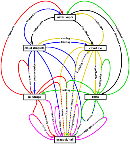
Fig. 7. An example of schematic summarizing for a given one-moment microphysical parametrization, showing the selected water categories or species, with arrows indicating the different processes operating among these species. The colour of an arrow refers to the species that is transformed by a process (black: water vapour, blue: cloud droplets, red: raindrops, yellow: cloud ice, green: snow, pink: graupel/hail), and when two species are concerned, the arrow is two-coloured (© Copyright Axel Seifert, reproduced with permission).

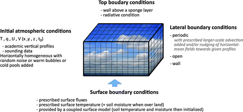
Fig. 8. Schematic of common choices of initial and boundary conditions in LES and CRMs.

Fig. 8. Schematic of common choices of initial and boundary conditions in LES and CRMs.

Fig. 9. Intercomparison of simulations of a mature squall-line performed with four distinct CRMs: the horizontal structure of the observed convective system is shown with a cross-section of radar reflectivity at 500 m above the surface in (a) and with simulated specific rain water (qr) at 1.4 km above the surface (b1–b4) – adapted from Redelsperger et al. (Citation2000a), © Copyright 2000 Royal Meteorological Society (RMS).
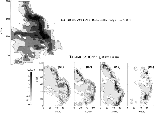
Fig. 9. Intercomparison of simulations of a mature squall-line performed with four distinct CRMs: the horizontal structure of the observed convective system is shown with a cross-section of radar reflectivity at 500 m above the surface in (a) and with simulated specific rain water (qr) at 1.4 km above the surface (b1–b4) – adapted from Redelsperger et al. (Citation2000a), © Copyright 2000 Royal Meteorological Society (RMS).

Fig. 10. Horizontal cross-sections of vertical velocity at 3 km above the surface in squall-line simulations differing in the choice of the constant Ck appearing in the formulation of the eddy diffusivity of the turbulent scheme ((a): Ck = 0.1, (b): Ck = 0.15, (c): Ck = 0.2). In these cross-sections, the dashed line corresponds to the gust front, and the interval between isolines is 1 m s−1. They choice of Ck has an impact on the number, intensity and scale of the simulated convective cells: they become spuriously small, strong and numerous for Ck = 0.1, while the opposite is observed for Ck = 0.2. The corresponding power spectra density (d) shows that the spurious peak of energy building up at short wavelengths for Ck = 0.10 (solid line) disappears for higher values of Ck – adapted from Takemi and Rotunno (Citation2005), © Copyright 2005 AMS.
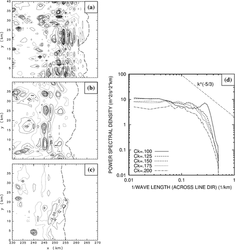
Fig. 10. Horizontal cross-sections of vertical velocity at 3 km above the surface in squall-line simulations differing in the choice of the constant Ck appearing in the formulation of the eddy diffusivity of the turbulent scheme ((a): Ck = 0.1, (b): Ck = 0.15, (c): Ck = 0.2). In these cross-sections, the dashed line corresponds to the gust front, and the interval between isolines is 1 m s−1. They choice of Ck has an impact on the number, intensity and scale of the simulated convective cells: they become spuriously small, strong and numerous for Ck = 0.1, while the opposite is observed for Ck = 0.2. The corresponding power spectra density (d) shows that the spurious peak of energy building up at short wavelengths for Ck = 0.10 (solid line) disappears for higher values of Ck – adapted from Takemi and Rotunno (Citation2005), © Copyright 2005 AMS.

Fig. 11. Intercomparison of CRM simulations of 14-day mean profiles of temperature (a) and (b) water vapour mixing ratio biases relative to observations and convective downdraught (c) and updraught (d) defined in the same way in each run – each line corresponds to one model and the thick dashed lines in (c) and (d) are the average of CRM profiles – adapted from Xu et al. (Citation2002), © Copyright 2002 RMS.
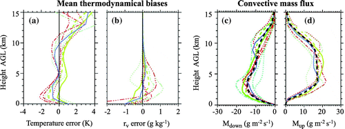
Fig. 11. Intercomparison of CRM simulations of 14-day mean profiles of temperature (a) and (b) water vapour mixing ratio biases relative to observations and convective downdraught (c) and updraught (d) defined in the same way in each run – each line corresponds to one model and the thick dashed lines in (c) and (d) are the average of CRM profiles – adapted from Xu et al. (Citation2002), © Copyright 2002 RMS.

Fig. 12. A snapshot of cloud albedo associated with (a) closed and (b) open cellular structures simulated with LES. The two simulations only differ in the initial concentration of aerosol with a high concentration favouring non-precipitating clouds in (a) and a low concentration favouring drizzle in (b) – adapted from Feingold et al. (Citation2010), © Copyright 2010 Nature.
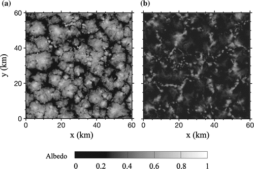
Fig. 12. A snapshot of cloud albedo associated with (a) closed and (b) open cellular structures simulated with LES. The two simulations only differ in the initial concentration of aerosol with a high concentration favouring non-precipitating clouds in (a) and a low concentration favouring drizzle in (b) – adapted from Feingold et al. (Citation2010), © Copyright 2010 Nature.

Fig. 13. Time sequence of four successive vertical cross-sections centred on the upper part of a growing cloud, with a 1-min frequency, starting to = 7.5 min after the initiation of the cloud. Arrows indicate wind in the cross-section. The contour delineates the cloud, defined as the area where the liquid water mixing ratio rc is lower than 0.01 g kg−1. The shading indicates the mixing ratio of a tracer rt introduced at the time of the first snapshot uniformly in a layer extending from 1100 to 1200 m at a 1 g kg−1 concentration; Starting at t = to + 1 min (b), the cloudy air penetrates and deforms this layer, and transports the tracers upwards, mainly on the edges of the cloud – adapted from Zhao and Austin (Citation2005), © Copyright 2005 AMS.

Fig. 13. Time sequence of four successive vertical cross-sections centred on the upper part of a growing cloud, with a 1-min frequency, starting to = 7.5 min after the initiation of the cloud. Arrows indicate wind in the cross-section. The contour delineates the cloud, defined as the area where the liquid water mixing ratio rc is lower than 0.01 g kg−1. The shading indicates the mixing ratio of a tracer rt introduced at the time of the first snapshot uniformly in a layer extending from 1100 to 1200 m at a 1 g kg−1 concentration; Starting at t = to + 1 min (b), the cloudy air penetrates and deforms this layer, and transports the tracers upwards, mainly on the edges of the cloud – adapted from Zhao and Austin (Citation2005), © Copyright 2005 AMS.

Fig. 14. Horizontal cross-section of potential temperature anomaly (a), vertical velocity (b) and wind speed (c) close to the surface, from a LES of deep convection over land. The figures illustrate the properties of the convectively generated cold pools: pools of negative temperature anomalies (a) with strong upward motion at their front – narrow orange stripes in (b) – and horizontal wind gusts – green and blue zones in (c).
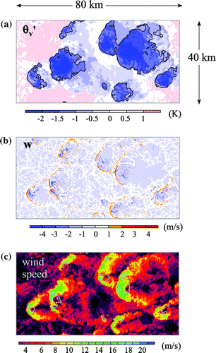
Fig. 14. Horizontal cross-section of potential temperature anomaly (a), vertical velocity (b) and wind speed (c) close to the surface, from a LES of deep convection over land. The figures illustrate the properties of the convectively generated cold pools: pools of negative temperature anomalies (a) with strong upward motion at their front – narrow orange stripes in (b) – and horizontal wind gusts – green and blue zones in (c).

Fig. 15. Comparison of conceptual schemes of turbulent mixing in parametrized shallow cumulus clouds when using either (a) weak and equal values of entrainment and detrainment rates ε and δ, or (b) stronger values of both with Δ > ε, as suggested by LES. The length and width of the arrows indicate the strength of mass fluxes. In (a), there is hardly any horizontal exchange between cloud air (within the cylinder) and its surrounding up to cloud top where detrainment is then massive, while in (b), the enhanced lateral mixing and the fact that detrainment dominates over entrainment over the whole cloud depth leads to a decrease of the convective mass flux with height (represented by a cone shape) and to much less detrainment at cloud top – adapted from Siebesma and Holtslag (Citation1996), © Copyright 1996 AMS.
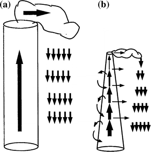
Fig. 15. Comparison of conceptual schemes of turbulent mixing in parametrized shallow cumulus clouds when using either (a) weak and equal values of entrainment and detrainment rates ε and δ, or (b) stronger values of both with Δ > ε, as suggested by LES. The length and width of the arrows indicate the strength of mass fluxes. In (a), there is hardly any horizontal exchange between cloud air (within the cylinder) and its surrounding up to cloud top where detrainment is then massive, while in (b), the enhanced lateral mixing and the fact that detrainment dominates over entrainment over the whole cloud depth leads to a decrease of the convective mass flux with height (represented by a cone shape) and to much less detrainment at cloud top – adapted from Siebesma and Holtslag (Citation1996), © Copyright 1996 AMS.

Fig. 16. An illustration of the sensitivity of the spatial structure (or organization) of deep tropical convection to the coupling with physical processes in convective radiative equilibrium (CRE) simulations. The plots show the water vapour mixing ratio at the lowest model level for (a) a reference simulation, (b) a simulation where surface fluxes do not respond to mesoscale fluctuations of the surface wind and (c) a simulation where radiative processes are prescribed instead of computed from the thermodynamical profiles and cloud field. The domain is replicated four times so that each panel represents a 200 km × 200 km square – adapted from Tompkins and Craig (Citation1998), © Copyright 1998 RMS.
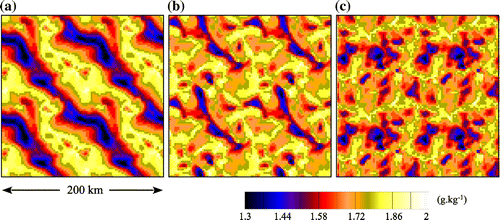
Fig. 16. An illustration of the sensitivity of the spatial structure (or organization) of deep tropical convection to the coupling with physical processes in convective radiative equilibrium (CRE) simulations. The plots show the water vapour mixing ratio at the lowest model level for (a) a reference simulation, (b) a simulation where surface fluxes do not respond to mesoscale fluctuations of the surface wind and (c) a simulation where radiative processes are prescribed instead of computed from the thermodynamical profiles and cloud field. The domain is replicated four times so that each panel represents a 200 km × 200 km square – adapted from Tompkins and Craig (Citation1998), © Copyright 1998 RMS.

Fig. 17. Snapshots of clouds (grey volumes) and near-surface air temperature (shading) in two convective–radiative equilibrium CRM runs, one without wind shear (a) and the other with shear in the lower atmosphere (b). The presence of shear changes the spatial scale of convective patterns, with isolated cells replaced by squall-line-type systems – adapted from Muller (Citation2013), © Copyright 2013 AMS.
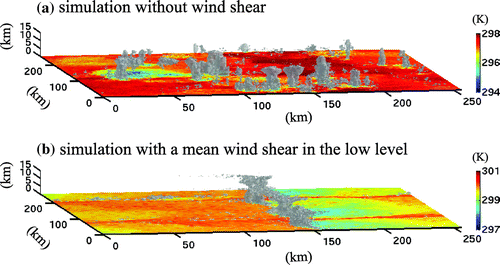
Fig. 17. Snapshots of clouds (grey volumes) and near-surface air temperature (shading) in two convective–radiative equilibrium CRM runs, one without wind shear (a) and the other with shear in the lower atmosphere (b). The presence of shear changes the spatial scale of convective patterns, with isolated cells replaced by squall-line-type systems – adapted from Muller (Citation2013), © Copyright 2013 AMS.