Recent subsurface North Atlantic cooling trend in context of Atlantic decadal-to-multidecadal variability

Figures & data

Fig. 1. Atlantic Multidecadal Oscillation indices for the period 1950–2015. Indices are created by area-averaging sea-surface-temperature and heat-content seasonal anomalies over the North Atlantic domain (75°W–5°W, Eq–60°N). (a) Unsmoothed and linearly detrended anomalies (shaded), linearly detrended and smoothed anomalies (dashed line), and undetrended and smoothed anomalies (continuous line) from HadISST’s SSTs, and linearly detrended and smoothed anomalies from ERV3b’s SSTs (dash-dot-dot line); units are in K. Correlation between the AMO smoothed indices from HadISST and ERV3b is 1. Note the levelling effect that the detrending has on the index by comparing the continuous and dashed lines. (b) Undetrended smoothed SST (from HadISST data set – thick black line) and ocean HC-based normalized AMO indices (from EN4.2.0 – colour lines). Normalization is done by dividing the smoothed index by its standard deviation in units of K for the SST index and J m⁻² for the AMO-HC indices as shown in the inset. Heat-content indices are calculated for the following layers of increasing depth: 5–149 m (thin grey line), 5–315 m (thin light blue line), 5–657 m (thick navy blue line), 5–968 m (thin dark red line), 5–1615 m (thin long-dash red line); the unsmoothed AMO index is drawn with the heavy black line. (c) Profiles of lead/lag correlations between the smoothed surface AMO index (HadISST) and smoothed detrended subsurface temperature anomalies in the 45°N–60°N and 30°N–45°N latitude bands; vertical axis is depth in m, horizontal axis is lead/lag in years and red/blue shading corresponds to positive/negative correlations; the grey stippling denotes significant grid points at the 95% confidence level based on a 2-tailed Student’s t-test.

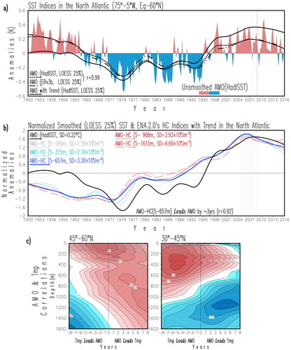
Fig. 2. Lead/lag regressions on detrended SST, subsurface temperature and salinity of the normalized smoothed (LOESS25%) AMO-HC (5–657 m) index at 2-year intervals for the period 1950–2015. Left column shows the regressed SST anomalies (HadISST), while the central and right columns show the depth-latitude regressed temperature and salinity anomalies (EN4.2.0) along the 35°W meridian; temperature anomalies are in units of 10⁻¹ K and salinity are with no units. Time runs down as indicated by the long red arrow to the right. Red/blue shading corresponds to positive/negative anomalies. Solid black lines in the left column panels mark the climatological annual mean position of the subpolar and subtropical gyres using the −0.4 m and +0.4 m absolute dynamic topography values, respectively, and the dashed black line tracks the climatological annual-mean position of the North Atlantic current through the −0.1 m topographic contour from AVISO altimetry. Solid navy blue lines display the climatological, long-term means, in SST, subsurface temperatures and salinity; temperatures are displayed every 2 °C and salinity every 0.4 units. The grey stippling denotes significant grid points at the 95% confidence level based on a 2-tailed Student’s t-test.

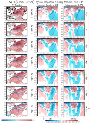
Fig. 3. Area-averaged HC seasonal anomalies in the North Atlantic (75°W–5°W, Eq–60°N – AMO-HC indices) from different data sets: EN4.2.0 (black line) for the 5–567 m layer, and Ishii (red line), and NODC (navy-blue line) for the 0–700 m layer. Anomalies are calculated with respect to the common 1981–2010 climatology. Units are in 10⁸ J m⁻².

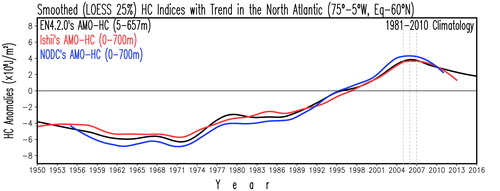
Fig. 4. Linear trends of the upper-ocean HC in EN4.2.0 and Ishii data sets. Trends are displayed for the period 1985–2005 from (a) the 5–657 m layer from EN4.2.0, and (b) the 0–700 m layer from the Ishii data set. The period 1985–2005 corresponds to the warming period observed in the AMO and AMO-HC indices seen in Fig. 1. Red/blue shading corresponds to positive/negative trends. Units are in 10⁸ J m⁻²/year. Solid black lines mark the climatological annual mean position of the subpolar and subtropical gyres using the −0.4 m and +0.4 m absolute dynamic topography values, respectively, and the dashed black line tracks the climatological annual-mean position of the North Atlantic current through the −0.1 m topographic contour from AVISO altimetry. The grey stippling denotes significant grid points at the 95% confidence level based on a 2-tailed Student’s t-test.

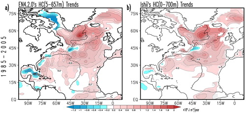
Fig. 5. Decadal linear trends in the upper-ocean HC and vertically averaged salinity for the 5–657 m layer before and after 2006 from EN4.2.0. Trends in HC are displayed in (a) for the period 1996–2005 and (b) for the period 2005–2015. Similarly, trends in salinity are displayed in (c) for the period 1996–2005 and d) for the period 2005–2015. The period 1996–2005 corresponds to the warming period observed in the AMO and AMO-HC indices, while the period 2005–2016 corresponds to the cooling period seen in Fig. 1. Red/blue shading corresponds to positive/negative trends in units of 10⁸ J m⁻²/year for HC and in units of 10⁻²/year in salinity. Solid black lines mark the climatological annual mean position of the subpolar and subtropical gyres using the −0.4 m and +0.4 m absolute dynamic topography values, respectively, and the dashed black line tracks the climatological annual mean position of the North Atlantic current through the −0.1 m topographic contour from AVISO altimetry. The grey stippling denotes significant grid points at the 95% confidence level based on a 2-tailed Student’s t-test.

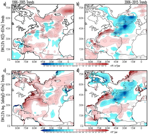
Fig. 6. Decadal trends at the atmosphere–ocean interphase before and after 2006. Panels in the left column show trends for the period 1996–2005, those in the right column for the period 2006–2010. Trends in mean sea level pressure are in panels (a) and (b) in units of 10⁻² h Pa/year from HadSLP2; trends in wind speed at 10 m are in panels (c) and (d) in units of 10⁻² m s⁻¹/year from OAFlux; trends in sensible plus latent heat flux are in panels (e) and (f) in units of Wm⁻²/year from OAFlux where positive trends indicate warming of the ocean; trends in SST are in panels (g) and (h) in units of 10⁻² K/year from HadISST. Red/blue shading corresponds to positive/negative trends. Solid black lines mark the climatological annual-mean position of the subpolar and subtropical gyres using the −0.4 m and +0.4 m absolute dynamic topography values, respectively, and the dashed black line tracks the climatological annual mean position of the North Atlantic current through the −0.1 m topographic contour from AVISO altimetry. Similar results are obtained by using NCEP/NCAR reanalysis data. The grey stippling denotes significant grid points at the 95% confidence level based on a 2-tailed Student’s t-test.

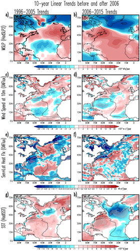
Fig. 7. Decadal mean anomalies and their change in upper HC (5–657 m) during three different decades from EN4.2.0. Panels in the left column are for the 1965–1974 decade, panels in the central column for the 1996–2005 decade, and panels in the right column are for the 2006–2015 decade. Mean anomalies are in panels (a), (b) and (c) in units of 10⁸ J m⁻². Tendencies in mean 10-year anomalies between two consecutive periods are in (d) 1965–1974 and 1964–1973, (e) 1996–2005 and 1995–2004 and (f) 2006–2015 and 2005–2014 in units of 10⁸ J m⁻². Red/blue shading corresponds to positive/negative anomalies and their change. Solid black lines mark the climatological annual mean position of the subpolar and subtropical gyres using the −0.4 m and +0.4 m absolute dynamic topography values, respectively, and the dashed black line tracks the climatological annual-mean position of the North Atlantic current through the −0.1 m topographic contour from AVISO altimetry.

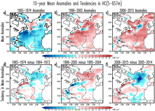
Fig. 8. Subpolar North Atlantic (SPNA) indices for the period 1950–2015. Indices are created by area-averaging anomalies over the subpolar domain (60°W–10°W, 45°N–60°N). (a) Normalized undetrended subpolar indices from HadISST’s SST anomalies (black heavy line), and EN4.2.0 HC anomalies for the layers 5–149 m (gray line), 5–315 m (thin light blue line), 5–657 m (thick blue line), 5–968 m (thin dark-red line) and 5–1615 m layer (thin long-dash red line). Normalization is done by dividing the smoothed index by its standard deviation in units of K for the SST index and 10⁸ J m⁻² for the heat content indices as shown in the inset. Maximum correlations between the surface and subsurface indices are displayed at the bottom right indicating that surface anomalies lead those at the subsurface over the subpolar region. Note that the indices in this region show cooling trends after 2006 which are larger than the all-basin indices in Fig. 1b. (b) Profiles of lead/lag correlations between smoothed detrended surface SPNA index and smoothed detrended subsurface temperature anomalies at the 45°N–60°N and 30°N–45°N latitude bands; the vertical axis is depth in m, horizontal axis is lead/lag in years, and red/blue shading corresponds to positive/negative correlations; the grey stippling denotes significant grid points at the 95% confidence level based on a 2-tailed Student’s t-test.

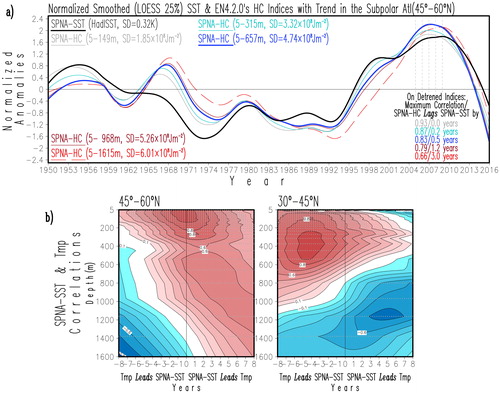
Fig. 9. Area-averaged wind anomalies and profiles of subsurface water property anomalies in the subpolar region (60°W–10°W, 45°N–60°N) from 1950 to 2015. (a) Wind-speed anomalies at 850 mb from the NCEP/NCAR reanalysis, (b) temperature (shaded) and salinity (contours) anomalies, (c) density (shaded) and salinity forced density anomalies (contours) and (d) density (shaded) and temperature forced density anomalies (contours). Salinity/temperature-forced density anomalies are calculated considering climatological temperature/salinity in the UNESCO formula. Wind speed is in ms⁻¹, temperature in K, salinity with no units, and densities are in kgm⁻³. Red/blue shading and continuous/dash lines correspond to positive/negative anomalies.

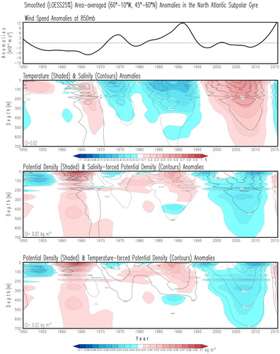
Fig. 10. The Gulf Stream index and its relationship to the upper-ocean HC (5–657 m)-based subpolar North Atlantic (SPNA) indices for the period 1954–2012. (a) Normalized unsmoothed GS index (shaded), smoothed (LOESS25%) GS index and undetrended smoothed (LOESS25%) SPNA HC index for the layers 5–657 m (blue line). (b) Map showing the regions where the GS and SPNA indices are defined. The GS index was obtained from temperature data at 200 m within the domain in the black rectangle (75°W–50°W, 33°N–43°N); the SPNA index used in (a) is area-averaged over the blue rectangle (60°W–10°W, 45°N–60°N); a western SPNA index is defined by area-averaging over the red rectangle (60°W–44°W, 45°N–60°N); a central SPNA index is defined by area-averaging over the green rectangle (44°W–27°W, 45°N–60°N); an eastern SPNA index is defined by area-averaging over the light blue rectangle (27°W–10°W, 45°N–60°N). (c) Lead/lag correlations between smoothed detrended GS index and SPNA HC-based indices. Note that the GS leads the subpolar indices and that the farther to the west the SPNA index is defined, the larger is the lag.

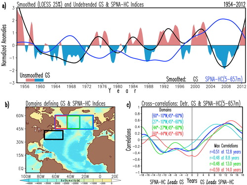
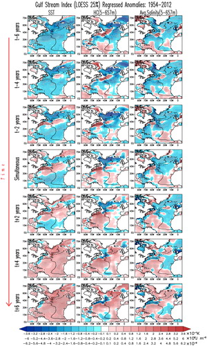
Fig. 11. Lead-lag regressions on detrended anomalies of the normalized smoothed (LOESS25%) GS index for the period 1954–2012. Panels in the left column show regressed SST anomalies in units of 10⁻¹ K, those in the central column display upper-ocean HC (5–657 m) anomalies in units of 10⁸ J m⁻², and panels in the right column show vertically averaged (5–657 m) salinity anomalies with no units at 2-year intervals from t − 6 years (top row) to simultaneous (central row) to t + 6 years (bottom row). Time runs down as indicated by the long red arrow to the left. Red/blue shading represents positive/negative anomalies. Solid black lines mark the climatological annual mean position of the subpolar and subtropical gyres using the −0.4 m and +0.4 m absolute dynamic topography values, respectively, and the dashed black line tracks the climatological annual-mean position of the North Atlantic current through the −0.1m topographic contour from AVISO altimetry. The grey stippling denotes significant grid points at the 95% confidence level based on a 2-tailed Student’s t-test.