Adding new evidence to the attribution puzzle of the recent water shortage over São Paulo (Brazil)

Figures & data

Fig. 1. (a) Geographical location of the São Paulo Cantareira water reservoir and the INMET climate stations in São Paulo State, (b) annual cycle of rainfall for 2013/14 and long-term mean for the period 1979–2004 from GPCP over São Paulo (averaged over the region 50°W to 45°W and 25°S to 20°S), (c) water storage volume (hm³) of Cantareira reservoir system for the period 1982 to early 2015 and (d) annual (July–June) and wet season (December, January and February) rainfall measured at the INMET stations in the State of São Paulo from 1961 to 2014.

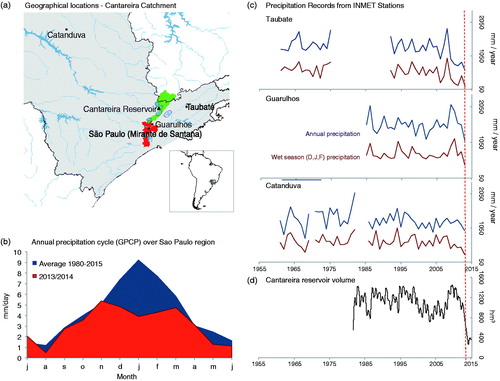
Table 1. Simulations carried out with HadAM3.

Simulation scenarios	Number of ensembles	SST	GHG	Land cover
1	6	Observed SST (HadISST)	Fixed at pre-industrial (280 ppm)	Fixed at 1870
2	6	Observed SST (HadISST)	Fixed at pre-industrial (280 ppm)	Time varying land cover (Meiyappan and Jain, 2012)
3	31	Observed SST (HadISST)	Increasing CO2	Time varying land cover (Meiyappan and Jain, 2012)

Table 2. List of CMIP5 climate models and ensemble outputs used in this study, simulation period, and research groups responsible for their development.

Models	Reference	Simulation period
CCSM4	Gent et al. (2011)	Jan 1850–Dec 2300
GFDL-ESM2M	Dunne et al. (2012, 2013)	Jan 1861–Dec 2100
HadGEM2-ES	Collins et al. (2011)	Dec1859–Dec 2299

Fig. 2. Annual and seasonal inflow into the Cantareira reservoir system for the period 1931–2015 based on SABESP records.

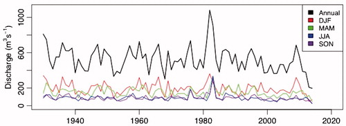
Fig. 3. Time latitude diagram of meridionally averaged (a) precipitation anomaly (GPCP), (b) Geopotential height anomaly (NCEP/NCAR), (c) Outgoing longwave radiation anomaly (NOAA) and (d) SST anomaly for the period July 2011 to December 2015. The precipitation has been averaged over São Paulo, i.e. 50°W to 40°W, whereas the other three variables have been averaged over the south Atlantic Ocean. Geopotential height and OLR have been averaged over 65°W to 40°W and SST has been averaged over 45°W to 10°W. The monthly anomalies of the climatic fields have been calculated with respect to the mean of the respective months during the whole period i.e. 1979–2004.

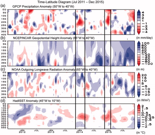
Fig. 4. December to February (DJF) rainfall anomaly (in mm/day) and SST (in °C) for 2013/14, 2014/15 and 2015/16. The rainfall has been adopted from GPCP (Adler et al., 2003) and the SST is from ERA-Interim (Dee et al., 2011). The top panel (a–c) shows the rainfall anomalies while the bottom panel (d–f) shows the SST anomalies. The geographical location of São Paulo city has been marked as green plus sign in all the subplots. We have chosen a box over the South Atlantic Ocean, which has been used to identify the similar occurrence of SST anomaly pattern in the future climate.

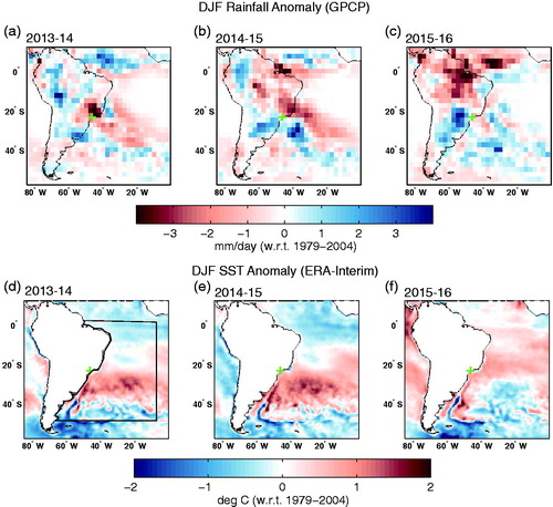
Fig. 5. Top panel: Moisture flux transport anomaly and SST anomaly (°C) obtained from ERA-Interim for (a) 2013/14 and (b) 2014/15 with respect to the mean of the respective fields during 1979–2004. The moisture flux transport has been plotted as vector field while the SST anomaly has been plotted as shaded. Bottom panel: moisture flux anomaly divergence for (c) 2013/14 and (d) 2014/15.

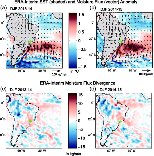
Fig. 6. Frequency distribution of DJF 2013/14 rainfall anomaly over the São Paulo region (25^oS to 20^oS and 50^oW to 45^oW) from HadCM3 simulations with observed land cover and observed GHG. Total 31 numbers of ensemble simulations were carried out by perturbing the initial conditions.

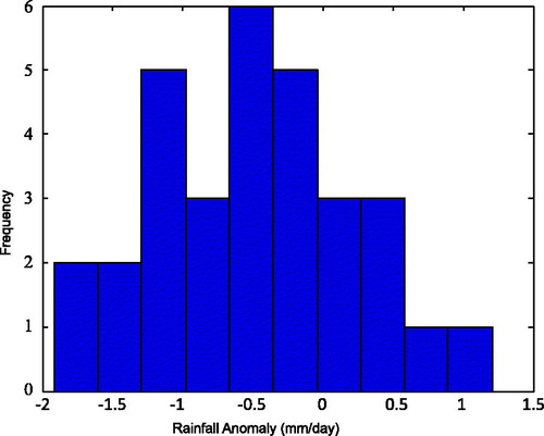
Fig. 7. DJF rainfall anomaly (mm/day) for 2013/14 (right panel) with respect to 1979–2004 from observations and HadAM3 simulations. Left and right columns represent observed and model simulated rainfall anomaly for 2013/14 respectively. (a) Observed rainfall from GPCP rainfall, b) simulation result of HadAM3 with fixed land cover (1870) and CO₂ fixed at preindustrial level (Scenario 1), (c) simulation results using HadAM3 with reconstructed time varying land cover (Meiyappan and Jain, 2012) and CO₂ fixed at preindustrial level (Scenario 2) and (d) simulation results using HadAM3 with reconstructed time varying land cover (Meiyappan and Jain, 2012) and observed GHGs increasing over time (Scenario 3). In this figure, the selection of the ensembles is based on criteria when the ensemble member simulates the rainfall anomaly over the São Paulo region (25^oS to 20^oS and 50^oW to 45^oW) less than –1 mm/day. Then the composite of these ensembles have been calculated and plotted above.

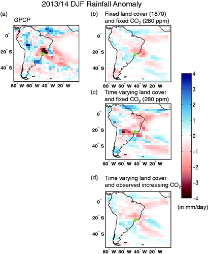
Fig. 8. (a) Pattern correlation of SST anomaly from ERA-Interim of DJF 2013/14 over south Atlantic (region shown in Fig. 3d i.e. 60°S to 0 and 42°W to 10°W) with SST anomaly in the other years. Red lines denote the years when the correlation is greater than or equal to 90th percentile and blue lines denote the years when the correlation is less than or equal to 10th percentile. (b) Frequency distribution of pattern correlation coefficients of ERA-Interim SST anomalies for 1979–2015.

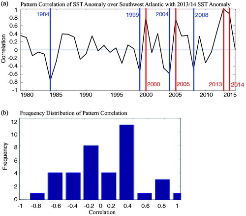
Fig. 9. DJF rainfall anomaly (GPCP), SST and moisture flux transport anomaly (ERA-Interim) during the years having correlation value greater than or equal to 90th percentile (Fig. 8) of the study period viz. 2000–01, 2005–05, 2013–14 and 2014–15. Top panel: rainfall anomaly for the years 2000–01 (a), 2005–06 (b), 2013–14 (c) and 2014–15 (d). Bottom panel: SST (in shaded) and moisture flux transport (in vector) anomaly for the years 2000–01 (e), 2005–06 (f), 2013–14 (g) and 2014–15 (h).

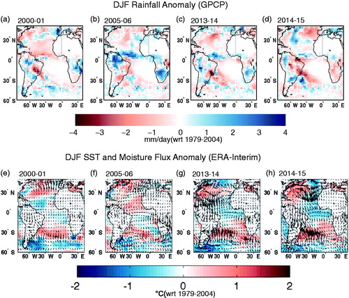
Fig. 10. Left panel represents the pattern correlation coefficients of SST anomaly of DJF 2013/14 from ERA-Interim with SST anomaly of other years for simulations with CCSM4 (a), GFDL-ESM2M (b) and HadGEM2-ES (c) for the period 1870–2100. Right panel represents the rainfall anomaly over the São Paulo region (25^oS to 20^oS and 50^oW to 45^oW) from CCSM4 (d), GFDL-ESM2M (e) and HadGEM2-ES (f) for the period 1870–2100. The blue and red curves represent historical and future periods in RCP8.5 scenario respectively. Black vertical lines in Fig. 8a–c indicate the years when the correlation value is more than 90th percentile and in Fig. 8d–f, the black vertical line shows the rainfall anomalies for the corresponding years.

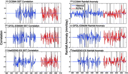
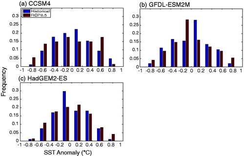
Fig. 11. Frequency distribution (normalized by division by total number of years) of pattern correlation coefficients (shown in Fig. 10) of SST anomalies for the simulations with CCSM4 (a), GFDL-ESM2M (b) and HadGEM2-ES (c) for the period 1870–2100. The blue and red bars represent historical and future periods in RCP8.5 scenario respectively.

Meiyappan, P. and Jain, A. K. 2012. Three distinct global estimates of historical land-cover change and land-use conversions for over 200 years. Front. Earth Sci. 6, 122–139. DOI:10.1007/s11707-012-0314-2.

 Web of Science ®Google Scholar

Gent, P. R., Danabasoglu, G., Donner, L. J., Holland, M. M., Hunke, E. C. and co-authors. 2011. The community climate system model version 4. J. Climate 24, 4973–4991. DOI:10.1175/2011JCLI4083.1.

 Web of Science ®Google Scholar

Dunne, J. P., John, J. G., Adcroft, A. J., Griffies, S. M., Hallberg, R. W. and co-authors. 2012. GFDL’s ESM2 global coupled climate–carbon earth system models. Part I: physical formulation and baseline simulation characteristics. J. Climate 25, 6646–6665. DOI:10.1175/JCLI-D-11-00560.1.

 Web of Science ®Google Scholar

Dunne, J. P., John, J. G., Shevliakova, E., Stouffer, R. J., Krasting, J. P. and co-authors. 2013. GFDL’s ESM2 global coupled climate–carbon earth system models. Part II: carbon system formulation and baseline simulation characteristics. J. Climate 26, 2247–2267. DOI:10.1175/JCLI-D-12-00150.1.

 Web of Science ®Google Scholar

Collins, W. J., Bellouin, N., Doutriaux-Boucher, M., Gedney, N., Halloran, P. and co-authors. 2011. Development and evaluation of an earth system model HadGEM2. Geosci. Model Dev. 4, 1051–1062. DOI:10.5194/gmd-4-1051-2011.

 Web of Science ®Google Scholar

Adler, R. F., Huffman, G. J., Chang, A., Ferraro, R., Xie, P.-P. and co-authors. 2003. The version 2 global precipitation climatology project (GPCP) monthly precipitation analysis (1979–Present). J. Hydrometeor. 4, 1147–1167. DOI:10.1175/1525-7541(2003)004<1147:TVGPCP>2.0.CO;2.

 Web of Science ®Google Scholar

Dee, D. P., Uppala, S. M., Simmons, A. J., Berrisford, P., Poli, P. and co-authors. 2011. The ERA-Interim reanalysis: configuration and performance of the data assimilation system. Quar. J. Royal. Meteorol. Soc. 137, 553–597. DOI:10.1002/qj.828.

 Web of Science ®Google Scholar