Figures & data
Fig. 1. Selected fields associated with the basic state. (a) The azimuthal velocity vb (colour), density potential temperature (solid black contours; K) and Exner function Πb (solid white contours). (b) A measure of gradient imbalance [
defined by Eq. (27)]. (c) The potential vorticity distribution. (d) The relative vertical vorticity distribution. (e) The radial vorticity (contours) and azimuthal vorticity (colour) distributions. The solid yellow and dashed white curves in (b)–(e) correspond to the principal AM isoline, which is commonly shown for spatial reference in the contour plots of this paper. Note that vbm is located where the radius of the isoline is minimised.
![Fig. 1. Selected fields associated with the basic state. (a) The azimuthal velocity vb (colour), density potential temperature θρb (solid black contours; K) and Exner function Πb (solid white contours). (b) A measure of gradient imbalance [Δgb defined by Eq. (27)]. (c) The potential vorticity distribution. (d) The relative vertical vorticity distribution. (e) The radial vorticity (contours) and azimuthal vorticity (colour) distributions. The solid yellow and dashed white curves in (b)–(e) correspond to the principal AM isoline, which is commonly shown for spatial reference in the contour plots of this paper. Note that vbm is located where the radius of the isoline is minimised.](/cms/asset/1a01f02f-2d7d-4840-98c3-c423abc64ad5/zela_a_1525245_f0001_c.jpg)
Fig. 2. The secondary circulation of the basic state. (a) Magnitude (colour) and streamlines of the velocity field (ub, wb) in the r-z plane. The streamlines are shaded white or black if the magnitude of the local velocity vector is respectively less than or greater than 5 m s−1. The dashed black curve is the principal AM isoline. (b) Magnified view of the secondary circulation in (a) in the lower troposphere.
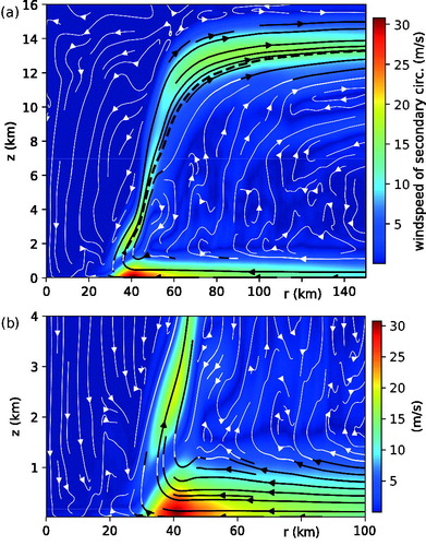
Fig. 3. The moist-thermodynamic structure of the basic state, illustrated primarily by the distributions of relative humidity (shading) and for liquid-only condensate (dashed black-and-white contours; J kg−1 K–1). The dotted blue curve is a selected contour of
computed under the assumption of ice-only condensate. The red curve is the principal AM isoline. The cyan curve traces the freezing/melting level across the vortex.
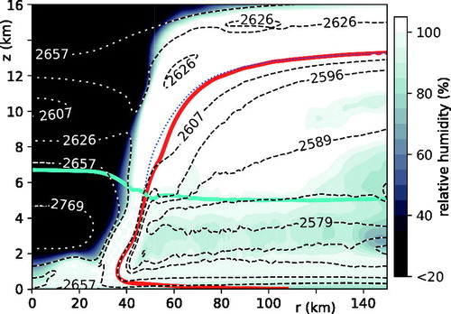
Fig. 4. Distributions of for (a)
and (b)
. The dashed white curves in (a) and (b) correspond to the principal AM isoline.
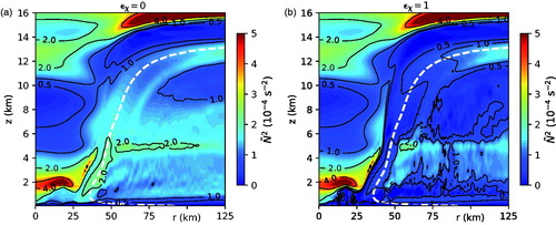
Fig. 5. Horizontal (colour) and vertical (solid contours) momentum eddy diffusivities in the middle-to-lower tropospheric core of the simulated tropical cyclone. The dashed curve is the principal AM isoline.
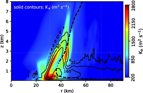
Fig. 6. Complex eigenfrequency λ of the n = 2 MUM of the simulated tropical cyclone of Section 4 versus the diabatic forcing parameter . The real (blue) and imaginary (red) parts of the eigenfrequency are normalised to their respective values (
s−1 and
s−1) obtained for
. The absence of a discernible instability precludes the plotting of data for
. Note that the positive ratio
represents a nondimensional magnitude of the oscillation frequency; the actual value of λI is negative. All results depicted here and in are for systems in which turbulent transport is parameterized with
.
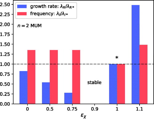
Fig. 7. (a)–(c) Basic inner-core structure of the n = 2 MUM for . (a) Vertical slices of the velocity perturbations in the azimuthal direction (colour) and in the r-z plane (vectors). (b) Vertical slices of the perturbations of density potential temperature (colour) and the Exner function (contours). (c) Vertical slice of the perturbation to diabatic forcing (colour) and contours of its maximum value along an azimuthal circuit. (d)–(f) As in (a)–(c) but for
. The yellow curve in each plot is the principal AM isoline. The slices in (a, b, d, e) are at an azimuth where
is maximised. The colour slices in (c) and (f) are at an azimuth where
is maximised.
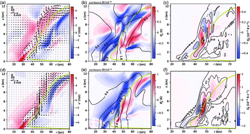
Fig. 8. (a)–(c) Maximum values over (
) of (a) the vertical vorticity perturbation, (b) the magnitude of the horizontal vorticity perturbation, and (c) the divergence of the horizontal velocity perturbation of the n = 2 MUM for
. (d)–(f) As in (a)–(c) but for
. The yellow curve in each plot is the principal AM isoline.
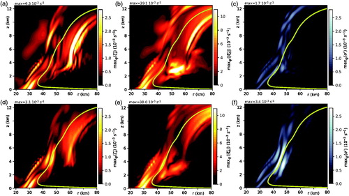
Fig. 9. (a) Intrinsic frequency of the n = 2 MUM normalised to the nominal inertial frequency
for the case in which
. The dashed green contours show where the intrinsic frequency is zero. The white area marked with an asterisk coincides with a region where
and the normalisation frequency is imaginary. The solid black contours of the amplitude (maximum over
) of
are shown for reference. (b) As in (a) but for
.
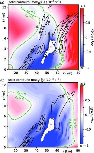
Fig. 10. (a, b) Slices of the vertical velocity perturbation of the n = 2 MUM in (a) the inner core and (b) the outer region of the vortex for the case in which . The dotted black contours in (a) correspond to
. The solid (dashed) white contours in (b) correspond to
(−7) cm s−1. Note that the units of the colorbar labels differ between (a) and (b). (c, d) As in (a, b) but for
. In all plots, the dashed black contour corresponds to the principal AM isoline. The azimuth of the top (bottom) row of the figure is equivalent to that of (7d).
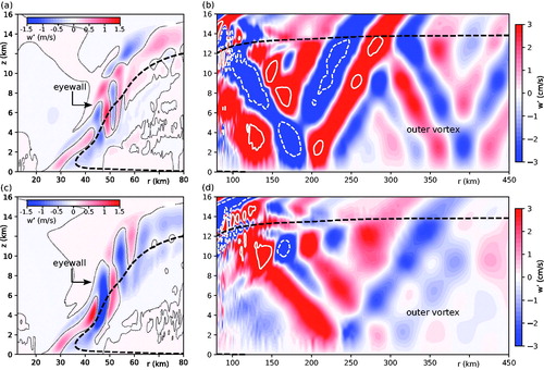
Fig. 11. (a) The symmetric velocity perturbation that attends the growth of the n = 2 MUM for the case in which . Colours depict v0 whereas vectors depict (u0, w0). (b) The perturbation of kinetic energy density associated with the n = 2 MUM and the attendant symmetric modification of the vortex for the case in which
. The perturbation is expressed as a positive or negative percentage of the local kinetic energy density of the basic state. The dotted black contours correspond to
. (c) The distribution of
associated with the n = 2 MUM for the case in which
. The white and black contours correspond to
J m−3. (d)–(f) As in (a)–(c) but for
. The yellow or red curve in each plot is the principal AM isoline. The thick black or blue line drawn from the location of vbm to the surface [in all plots but (b) and (e)] shows where vb is maximised with respect to variation of r in the boundary layer. The thin black curves in (a) and (d) trace the edges of the unperturbed eyewall updraft, where wb is 2.5% of its maximum positive value.
![Fig. 11. (a) The symmetric velocity perturbation that attends the growth of the n = 2 MUM for the case in which ϵχ=0.5. Colours depict v0 whereas vectors depict (u0, w0). (b) The perturbation of kinetic energy density associated with the n = 2 MUM and the attendant symmetric modification of the vortex for the case in which ϵχ=0.5. The perturbation is expressed as a positive or negative percentage of the local kinetic energy density of the basic state. The dotted black contours correspond to δKE=0. (c) The distribution of KEn associated with the n = 2 MUM for the case in which ϵχ=0.5. The white and black contours correspond to KEn=[0.6,3.2,6.3,13,19] J m−3. (d)–(f) As in (a)–(c) but for ϵχ=1. The yellow or red curve in each plot is the principal AM isoline. The thick black or blue line drawn from the location of vbm to the surface [in all plots but (b) and (e)] shows where vb is maximised with respect to variation of r in the boundary layer. The thin black curves in (a) and (d) trace the edges of the unperturbed eyewall updraft, where wb is 2.5% of its maximum positive value.](/cms/asset/ef77dadc-8971-4e13-a5aa-e9777d181289/zela_a_1525245_f0011_c.jpg)
Fig. 12. Domain integrals of the individual contributions to [Equations (30b)–(30g)] and their sum for the n = 2 MUM with (left to right)
to 1.1. The value of each integral is normalised to that of
. The contributions from AFX and PFX are combined into APFX. The PC contribution is decomposed into the radial shear component proportional to
(r, dark red) and the vertical shear component proportional to
(v, light red). The TRB contribution is decomposed into the primary part attributable to turbulent dissipation (dark cyan) and the much smaller part attributable to sponge damping (light cyan cap).
![Fig. 12. Domain integrals of the individual contributions to ∂tKEn [Equations (30b)–(30g)] and their sum for the n = 2 MUM with (left to right) ϵχ=0 to 1.1. The value of each integral is normalised to that of ∂tKEn. The contributions from AFX and PFX are combined into APFX. The PC contribution is decomposed into the radial shear component proportional to ∂rΩb (r, dark red) and the vertical shear component proportional to ∂zvb (v, light red). The TRB contribution is decomposed into the primary part attributable to turbulent dissipation (dark cyan) and the much smaller part attributable to sponge damping (light cyan cap).](/cms/asset/ee83af2a-5b93-4fb0-8ebe-f40b24e24acb/zela_a_1525245_f0012_c.jpg)
Fig. 13. Variation of the complex eigenfrequency λ of the n = 2 MUM and SMUM with the small-scale turbulence parameter for systems with (top)
and (bottom)
. The real (blue) and imaginary (red) parts of each eigenfrequency are normalised to their respective values (
s−1 and
s−1) obtained for the MUM when
.
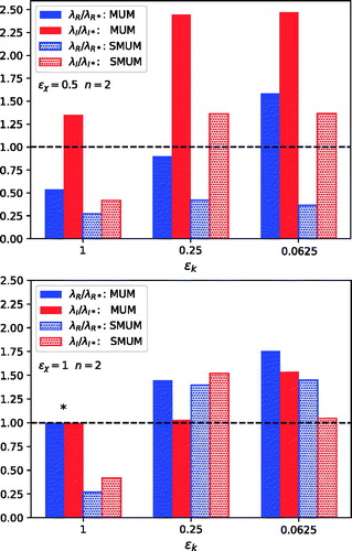
Fig. 14. (a) Spatial distribution of for the n = 2 MUM with
and
. The white and black contours correspond to
W m−3. (b) Domain integrals of the individual contributions to
for the n = 2 MUM with
and
. (c, d) As in (a, b) but for
and
. (e, f) As in (a, b) but for the n = 3 MUM with
and
. The red curves in (a, c, e) correspond to the principal AM isoline; the dashed green curves show where
; the blue lines show where vb is maximised with respect to variation of r in the boundary layer. The plots in (b, d, f) are completely analogous to those in .
![Fig. 14. (a) Spatial distribution of ∂tKEn=2λRKEn for the n = 2 MUM with ϵχ=0.5 and ϵk=0.0625. The white and black contours correspond to ∂tKEn=[0.1,0.5,1.0,2.0,4.0] 10−3 W m−3. (b) Domain integrals of the individual contributions to ∂tKEn for the n = 2 MUM with ϵχ=0.5 and ϵk=0.0625. (c, d) As in (a, b) but for ϵχ=1 and ϵk=0.0625. (e, f) As in (a, b) but for the n = 3 MUM with ϵχ=1 and ϵk=0.25. The red curves in (a, c, e) correspond to the principal AM isoline; the dashed green curves show where cφ=0; the blue lines show where vb is maximised with respect to variation of r in the boundary layer. The plots in (b, d, f) are completely analogous to those in Fig. 12.](/cms/asset/94eae0c1-d68c-49cd-b16d-4059da85e12f/zela_a_1525245_f0014_c.jpg)
Fig. 15. (a) Azimuthal wavenumber (n) dependence of the growth rate of the 2D MUM for several values of , as indicated in the legend. Computed MUMs with growth rates of order
s−1 or less (at high n and appreciable
) are excluded from the plot, because they are considered virtually neutral and have questionable accuracy. (b)
dependencies of the growth rates of the two most unstable 2D eigenmodes associated with an n = 2 perturbation. (c) As in (b) but for the oscillation frequencies. The extended blue ticks on the vertical axes of (b) and (c) mark the growth rate and oscillation frequency of the n = 2 MUM of the 3D system with
and
; the red ticks are the same but for
.
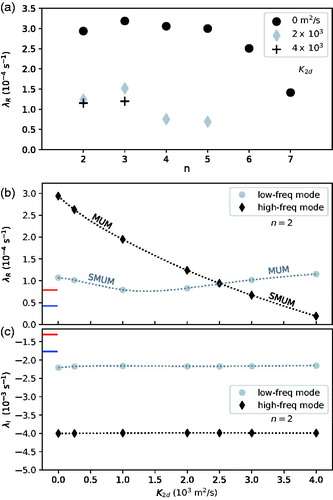
Fig. 16. (a) Vertical vorticity (red and blue), streamlines (black) and corotation circles (dashed green) of the low-frequency mode of the 2D system with m2 s−1. The streamline thickness is directly proportional to the local magnitude of the horizontal velocity perturbation
. (b) As in (a) but for the high-frequency mode. (c) As in (a) but for vertically averaged fields associated with the MUM of the 3D system with
and
; the averaging is over a 2 km layer adjacent to the sea-surface. (d) As in (c) but with the streamlines corresponding to the irrotational component of
. (e, f) As in (c, d) but for
; note that segments of the corotation circle can be found at the corners of both plots. In all subfigures, the axis labels x and y denote horizontal Cartesian coordinates measured from the center of the vortex.
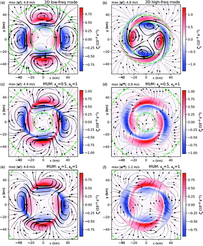
Fig. 17. Comparison between the prevailing instability modes of a tropical cyclone simulated with CM1 and two theoretical predictions. (a) Growth rate versus azimuthal wavenumber n as determined by (circles) 2D instability theory, (diamonds) 3D instability theory, and (squares) the pertinent 3D CM1 simulation of NS14. (b) As in (a) but for the oscillation frequency. The error bars are explained in the main text.
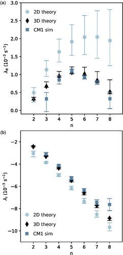
Fig. B1. Scatter plot of the complex eigenfrequencies of the n = 2 MUM in linear systems with (pink) and without (black) acoustic filtering. Different symbol shapes correspond to different combinations of and
as shown in the legend in the lower left corner of the graph.
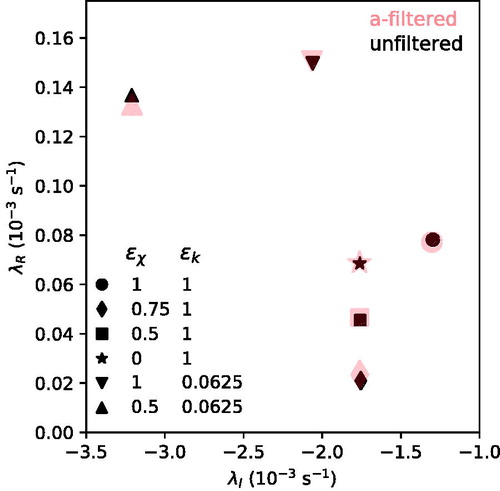
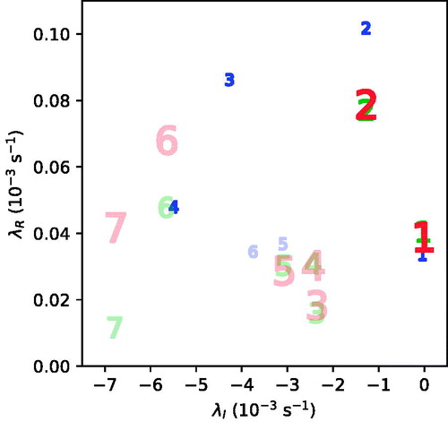
Fig. C1. Scatter plot of the complex eigenfrequencies of the MUMs of the tropical cyclone of Section 4 as determined by the 3D linear model with . The number associated with each data point denotes the value of the azimuthal wavenumber (n) of the MUM. Data is included for computations on G1 (small blue), G2 (medium green) and G4 (large red). Dark (light) symbols indicate modes with
maximised in the lower (middle) troposphere. Note that the G4 data correspond to eigenfrequencies nearest to those of the G2 MUMs, but the associated modes were not verified to dominate time-asymptotic perturbations on G4.