Large-scale secondary circulations in a limited area model – the impact of lateral boundaries and resolution

Figures & data

Table 1. Model configurations used for CCLM simulations. The shifts of the model boundaries are given as number of grid boxes, with positive values indicating a shift away from the centre of the domain.

Name	Horizontal resolution	Shift of lateral boundaries				Domain size	Filtered orography	Spectral nudging
		North	East	South	West
REF	0.165°	0	0	0	0	257 × 271	no	no
N − 64	0.165°	−64	0	0	0	257 × 207	no	no
N − 32	0.165°	−32	0	0	0	257 × 239	no	no
N + 32	0.165°	+32	0	0	0	257 × 303	no	no
N + 64	0.165°	+64	0	0	0	257 × 335	no	no
E − 64	0.165°	0	−64	0	0	193 × 271	no	no
E − 32	0.165°	0	−32	0	0	225 × 271	no	no
E + 32	0.165°	0	+32	0	0	289 × 271	no	no
E + 64	0.165°	0	+64	0	0	321 × 271	no	no
S − 64	0.165°	0	0	−64	0	257 × 207	no	no
S − 32	0.165°	0	0	−32	0	257 × 239	no	no
S + 32	0.165°	0	0	+32	0	257 × 303	no	no
S + 64	0.165°	0	0	+64	0	257 × 335	no	no
W − 64	0.165°	0	0	0	−64	193 × 271	no	no
W − 32	0.165°	0	0	0	−32	225 × 271	no	no
W + 32	0.165°	0	0	0	+32	289 × 271	no	no
W + 64	0.165°	0	0	0	+64	321 × 271	no	no
LARGE	0.165°	+125	+125	+125	+125	507 × 521	no	no
RES33	0.330°	0	0	0	0	129 × 136	no	no
RES66	0.660°	0	0	0	0	65 × 68	no	no
SN	0.165°	0	0	0	0	257 × 271	no	yes
FILT	0.165°	0	0	0	0	257 × 271	yes	no

Fig. 1. Results of the reference configuration REF based on temporal averages of the analysis period at the 500 hPa level. (a) ECHAM geopotential height (contour lines), wind vectors (arrows) and wind speeds (colours). (b) ECHAM geopotential height (contour lines), ensemble mean wind vector differences (arrows) and wind speed differences (colours) between CCLM and ECHAM. (c) ECHAM geopotential height (contour lines), ensemble mean wind vector differences (arrows) and geopotential height differences (colours) between CCLM and ECHAM. Green rectangles indicate region A (dashed green line) and B (solid green line). (d) ECHAM geopotential height (contour lines), ensemble mean wind vector differences (arrows) and ensemble standard deviation of geopotential height differences between CCLM and ECHAM (colours). The longest vector in b–d is 7.8 m/s.

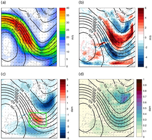
Fig. 2. As Fig. 1c, but for model configurations with shifted (a,c) eastern and (b,d) western model boundaries. Five vertical solid black straight lines (including the outermost boundary) represent the five different locations of each lateral boundary with a distance of 32 grid boxes.

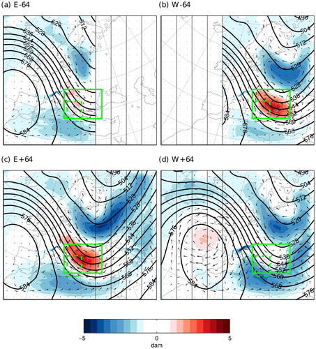
Fig. 3. As Fig. 1c, but for model configurations with shifted (a,b) northern and (c,d) southern model boundaries. Five horizontal solid black straight lines (including the outermost boundary) represent the five different locations of each lateral boundary with a distance of 32 grid boxes.

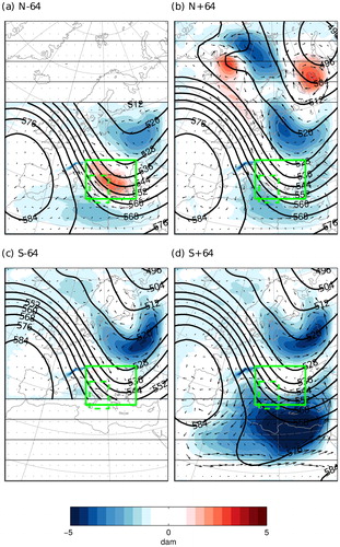
Fig. 4. (a) Area mean of region A of the ensemble mean (points) and standard deviation (error bars) of the norm of the of wind vector differences between CCLM and ECHAM and (b) area maximum of region B of the ensemble mean and standard deviation of the geopotential height differences between CCLM and ECHAM at 500 hPa for different model configurations.

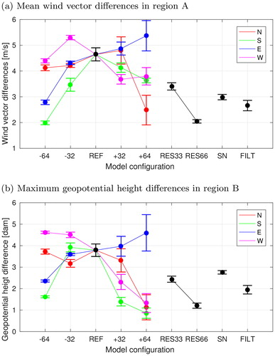
Fig. 5. (a) As Fig. 1c, but for model configuration LARGE. (b) As Fig. 1d, but for model configuration LARGE. (c) ECHAM fields as Fig. 1a, but for the domain of model configuration LARGE. (d) Variables as in Fig. 1a, but for the ensemble mean of the CCLM configuration LARGE. The area covered by the model configuration REF is indicated by rectangle in solid black lines.

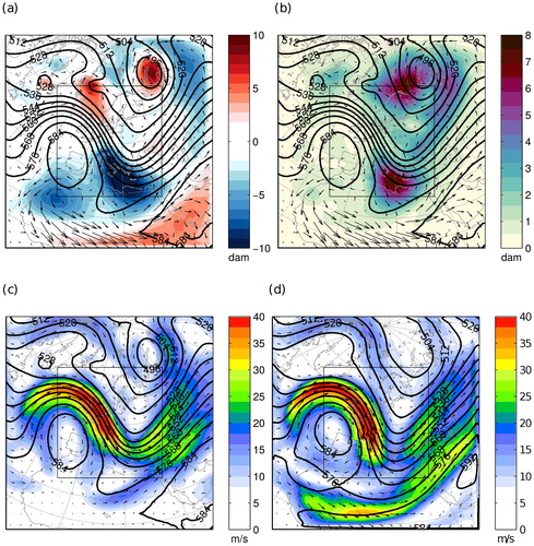
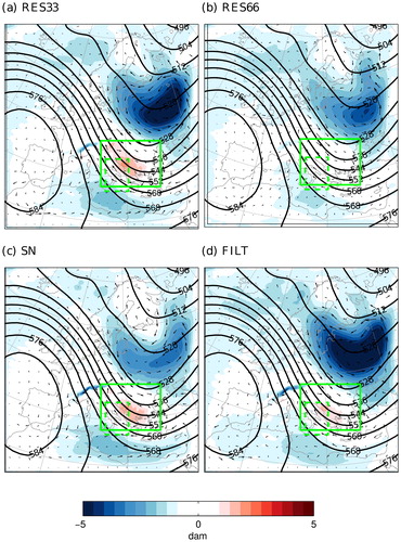
Fig. 6. As Fig. 1c, but for model configurations with different resolutions, spectral nudging and smoothed topography.