Probabilistic thunderstorm forecasting by blending multiple ensembles

Figures & data

Table 1. Forecast ranges used for the parameter tuning.

Ensemble name	Tuning ranges (h)
AromeEPS + AROLAG	12–30 every 6 h
AromeEPS + PEARP	24–42 every 6 h
PEARP + IFSens	42–60 every 6 h

Table 2. Coefficients s of the reliability calibration, diagnosed for each blend over 3 different months.

Blend name	AromeEPS + AROLAG	AromeEPS + PEARP	PEARP + IFSens
June 2018	0.165	0.208	0.314
July 2018	0.147	0.156	0.325
August 2018	0.160	0.147	0.249

Fig. 1. Left panel: Lightning flashes from the Météorage network (9 August 2018, 00UTC), the colours indicate the number of strokes per flash. Right panel: Pseudo-observations of thunderstorms (light bullets: non-occurrence, dark bullets: occurrence).

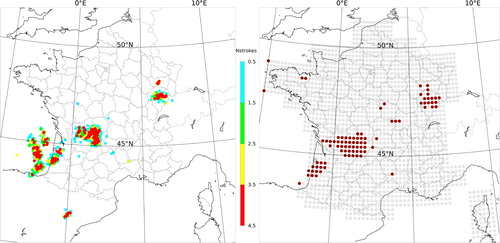
Fig. 2. Timings of the four ensembles considered in the paper, relative to the same 00UTC production base. The thick horizontal arrows indicate the forecasts runs (deterministic and ensembles); the dashed horizontal segments indicate forecast ranges that are computed but not used (some forecasts may also extend further into the future than represented here). Grey boxes and arrows indicate the ensembles and tuning windows used in each ensemble blend. The model grid resolution is given next to each ensemble name.

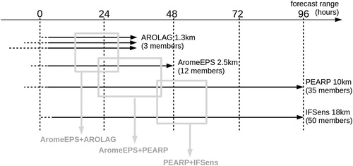
Fig. 3. ROC diagrams of the AromeEPS ensemble thunderstorm forecasts, without any post-processing (‘raw ensemble’), with the 20 km neighbourhood operator (‘neigh’), with neighbourhood and dressing operators (‘neigh + dress’, with d = 1), and with the neighbourhood operator with a re-tuned threshold u (‘neigh + thres’, made with u = 8, instead of 10 in the other curves). The diagrams are computed over June, July and August 2018 (i.e. 92 days), on forecast ranges from 12 to 42 h. The apparent differences between the ROC areas are significant at the 95% level. The respective ROC areas are 0.54, 0.72, 0.77, 0.74, and the ROC area with the combined neighbourhood, dressing operators and retuned threshold (curve not shown) is 0.78.

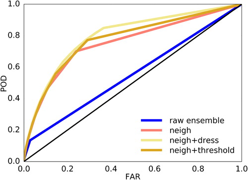
Fig. 4. 1D transects of the ROCA(r, d, w, u) surrogate function around the optimum, for the AromeEPS + AROLAG ensemble mix, over June 2018. The curves have been horizontally rescaled so that the optimum is at zero, values below (resp. above) the optimum have been linearly rescaled from their minimum (resp. maximum) search value to −1 (resp. +1).

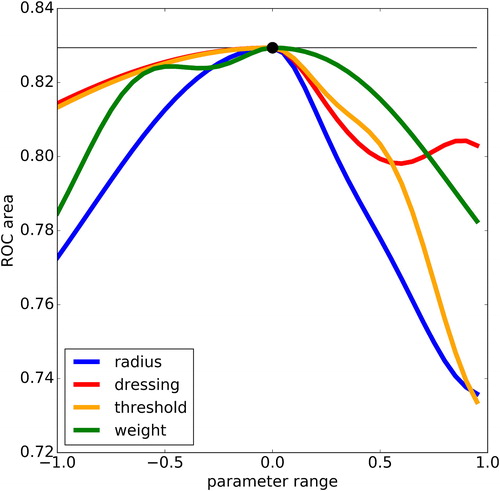
Fig. 5. Optimized values of the parameters (r, d, w, u) i.e. (radius, dressing, weight, threshold) for three ensemble blends, over 3 independent periods (June, July and August 2018). The blue bars show the values that optimize the ROCA area, the black vertical bars show the uncertainty interval that is implied by the optimization procedure.

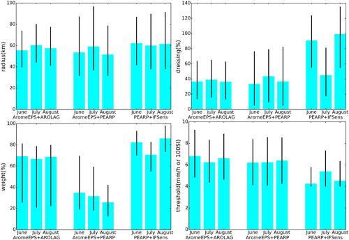
Fig. 6. Reliability diagrams for the AromeEPS + AROLAG blend where (r, d, w, u) have been optimized over June 2018. The curves are displayed before and after applying the reliability calibration procedure. The numbers indicate the sample size used to compute each point (K means 1000).

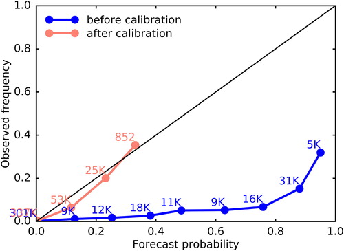
Fig. 7. Thunderstorm probability forecasts based on 8 August 2018, 00UTC and valid 24 h later, forecast by (from left to right) the raw Arome-EPS ensemble, the calibrated AromeEPS + AROLAG, AromeEPS + PEARP and PEARP + IFSens blends. The black disk indicates the city of Bordeaux.

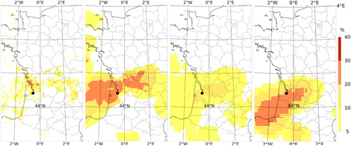
Fig. 8. Values of tuning parameters (r, d, u) i.e. (radius, dressing, threshold), independently optimized for each ensemble used in the blends. The optimization is done over June 2018. The graphical conventions are as in Fig. 5.

Fig. 9. ROC areas and potential economic values of the forecast thunderstorm probabilities, for the three ensemble blends (one per row) and their contributing ensembles. The plots are averaged over 92 days. The potential economic value diagrams (right column) are averaged over the same forecast ranges as the ROC areas (left). Bullets are plotted on the ROCA curves when the contributor score is statistically significant from the blend score.

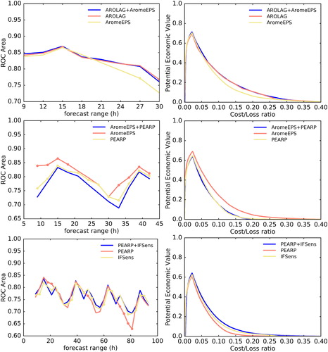
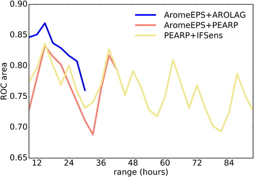
Fig. 10. ROC areas of the three blends, over their respective forecast ranges, averaged over 92 days.