A simple theory for the modulation of tropical instability waves by ENSO and the annual cycle

Figures & data

Fig. 1. (a) Hovmöller diagram of daily SST anomalies between 180° and 100°W (0°-6°N latitudinal average). The red and blue horizontal lines represent the longitudinal positions of the nodes used to generate TIW indices. Red (blue) nodes/lines are positive (negative). (b) $TI{W}_1(t)=\sum \pm \mathit{SST}\prime (t,\mathit{nodes})$ time series. (c) Global wavelet spectrum of TIW₁. See the mathematical definition of TIW₁ and TIW₂ indices in Section 2.

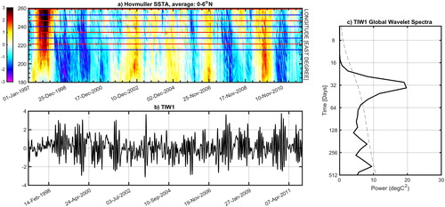
Fig. 2. (a) Regression of daily SST anomalies onto TIW₁ index (1997–2015). Dots denote the 95% statistical significance level. Black filled triangles and circles show the positions of longitudinal nodes (positive for circles, i.e. red lines on Fig. 1a, and negative for triangles, i.e. blue lines on Fig. 1a). The bottom right panel (b) is the (TIW₁, TIW₂) phase diagram. (c) Auto correlation of TIW₁-TIW₂ in black and cross correlation between TIW₁ and TIW₂ in red.

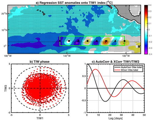
Fig. 3. (a) Annual cycle (monthly mean climatology) of the observed TIW amplitude (1997-2015) (black) and of the ensemble average of the 2^nd order TIW amplitude analytical solution inferred with different reasonable values of γ_A/γ₀ and γ_N/γ₀ ($0.2\le \left|\frac{{\gamma }_A}{{\gamma }_0}\right|,\left|\frac{{\gamma }_N}{{\gamma }_0}\right|\le 0.8$ ) and different versions of the model, i.e. using only a annually-varying TIW damping rate (TIWxAC) in red, using only an interannually-varying TIW damping rate (TIWxNino) in green and using both (TIWxTOT) in magenta. (b) Same but for the monthly variance of TIW amplitude. (c) FFT single-sided spectrum of the observed TIW amplitude (i.e. |Z| = TIW₁₂, black) and ensemble averaged of FFT single-sided amplitude spectra of the 2^nd order approximation of the TIW amplitude analytical solution for the different versions of the model (same colour code as (a)). The dashed blue line indicates the averaged spectrum of 5000 generations of a random red noise process. The Coloured vertical bands indicate select time scales: ENSO (2.5-5 years) in green, the Annual Cycle (AC, 340-390 days) in pink, the Semi Annual Cycle (SAC, 160-200 days) in orange, and the combination mode (C-MODE) in purple. Period: Jan 1^st 1997-Dec 31^st 2015.

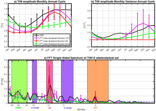
Fig. 4. (a) Average of (TIW₁-TIW₂) autocorrelations (in black) and (TIW₁,TIW₂) cross correlations (in red) logarithm for climatological years (i.e. neither El Niño nor La Niña years) between November and February. The black dotted line represents the best linear fit to these curves local maxima or in other words the estimation of TIWs propagation e-folding time during neutral years. Similarly, the green (magenta) dotted line represents the best linear estimation of TIWs propagation e-folding time for El Niño (La Niña) years. The red (blue) dotted line represents the best linear estimation of TIWs propagation e-folding time for extreme El Niño (La Niña) years. (b) The inverse of these e-folding times (in other words, TIWs growth rates) are represented as a function of the daily equatorial (2°S-4°N; 180°W-100°W) SST anomalies averaged during the corresponding periods and years (in red). The black curve is the same but for TIWs growth rates as a function of the meridional gradient of SST anomalies, i.e. the difference between the equatorial region average and the [7°N-13°N; 180°W-100°W] average. (c) Same as (a) but during different seasons of neutral years: Auto (black) and cross (red) correlations logarithm averaged during February-September. The corresponding e-folding time linear estimation is shown in the dotted black line. The green, respectively magenta, dotted line represents the best linear estimation of TIWs propagation e-folding time during the summer and fall (July-September), respectively spring and winter (February-April) of neutral years. (d) Same as (b) but the TIWs seasonal growth rates are shown as a function of the corresponding equatorial SST average in red and the meridional climatological SST gradient in black.

Fig. 5. (a) Individual members (thin Coloured lines) and ensemble average (thick blue line) of the daily TIW amplitude numerical solutions using the full TIWxTOT version of the model. The black line shows the observed daily TIW amplitude. The thick red line is the 2^nd order analytical solution of TIW amplitude. All time series are normalised and smoothed using a 50-days running mean. (b) Spectra of the observed and 2^nd order approximation of the analytical solution of TIW amplitude from different sensitivity experiments. Thick black lines for observation, red for the experiments using only a annually-varying TIW damping rate (TIWxAC), green for the experiments using only an interannually-varying TIW damping rate (TIWxNino) and magenta for the experiments using both (TIWxTOT). The dashed blue line indicates the averaged spectrum of 5000 generations of a random red noise process.

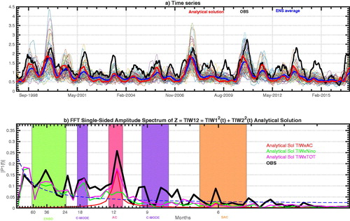
Fig. 6. (a) Spectra of the observed and ensemble average of TIW amplitude (Z = TIW12) simulated by different sensitivity experiments (the Coloured bands representing different typical timescales, see Fig. 5b caption). Thick black lines for observation, red for the experiments using only a annually-varying TIW damping rate (TIWxAC), green for the experiments using only an interannually-varying TIW damping rate (TIWxNino) and magenta for the experiments using both (TIWxTOT). The dashed blue line indicates the averaged spectrum of 5000 generations of a random red noise process. (b) Annual cycle of the observed (black line), the ensemble average (blue line) and the analytical solution (red) of TIW amplitude; the annual cycle of the model forcing is shown in green. (c) Scatter plot of simulated TIW amplitude (TIWxTOT ensemble average) versus the prescribed Niño3 forcing.

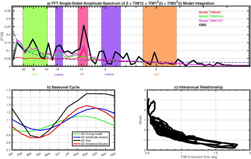
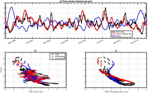
Fig. 7. (a) Observed interannual part (i.e. cleared from the 1997–2015 monthly mean climatology) of TIW amplitude (black) and interannual part of the analytical solution 2^nd order approximation of TIW amplitude (red) using the following set of parameters: γ₀ = 1/23 days⁻¹_; γ_A/γ₀ = 0.3; γ_N/γ₀ = −0.5 and γ_N³ = 0.007; The correlation between these two timeseries is 0.65. The blue line shows the Niño3 index. (b) Scatter plot of the nonlinear relationship between the observed interannual TIW amplitude and ENSO (Niño3 index); Red (summer/fall only) and blue (winter/spring only) dots highlight the seasonality of this relationship. (c) Same as (b) for the the nonlinear relationship between the 2^nd order approximation of the analytical solution of the interannual TIW amplitude and ENSO.