Nonlinear interaction of gravity and acoustic waves

Figures & data

Table 1. Definition of variables, symbols and operators.

x	Eastward distance
y	Northward distance
z	Altitude
t	Time
u	Zonal wind
v	Meridional wind
w	Vertical wind
$\mathit{V}={(u,v)}^T$	Horizontal wind vector
p	Pressure
ρ	Density
T	Temperature
R	Gas constant for dry air
cp	Specific heat at constant pressure
cv	Specific heat at constant volume
$\gamma =c_p/c_v$
$\kappa =R/c_p$
$T_0=243.878$ K	Temperature of the isothermal basic state
$L_x=4\times {10}^7\hspace{0.17em}\text{cos}({\varphi }_0)$ m	Zonal period
$L_y={10}^7$ m	Meridional period
zT = 18,000 m	Model’s top
$\Omega =2\pi /(24\times 60\times 60)$ s^−1	Earth’s rotation rate
${\varphi }_0=\pi /4$	Central latitude of $f-$ plane
$f=2\Omega \hspace{0.17em}\text{sin}({\varphi }_0)$	Coriolis parameter
g = 9.8 m s^−2	Earth’s gravitational acceleration
$C_S=\sqrt{\gamma R{T}_0}$	Linear sound wave speed
$\mathit{V}·\nabla h=u{\partial }_{x}h+v{\partial }_{y}h$
$\nabla ·\mathit{V}={\partial }_{x}u+{\partial }_{y}v$	Horizontal divergence

Fig. 1. Dispersion curves of inertia-acoustic (AI) and inertia-gravity (IG) waves corresponding to the first three baroclinic modes m = 1, 2, 3. All the curves are referred to the meridional index n = 1.

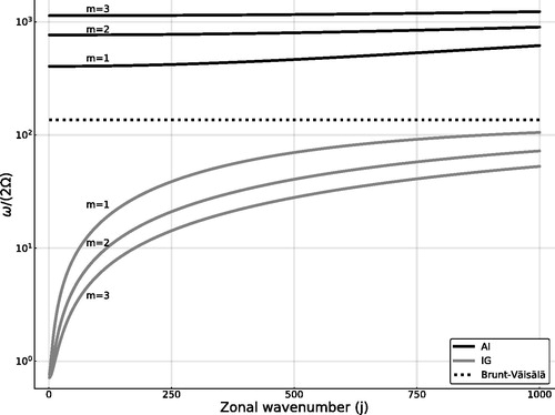
Fig. 2. Similar to Fig. 1, but only for the inertia-gravity waves (IG) and their corresponding dispersion curves obtained by hydrostatic approximation (H).

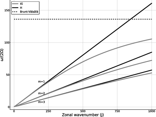
Table 2. Representative examples of interacting triads involving inertia-acoustic (IA) and inertia-gravity modes (IG).

Triad	Mode a	Mode b	Mode c	ωa	ωb	ωc	δabc	$i{\sigma }_a$	$i{\sigma }_b$	$i{\sigma }_c$
1	(1, 1, 1, IA)	(339, 1, 2, IG)	(340, 1, 1, IA)	5.89E–02	4.10E–03	6.30E–02	3.31E–05	–3.11E–01	–2.16E–02	–3.33E–01
2	(170, 1, 2, IG)	(169, 1, 2, IG)	(339, 1, 2, IG)	2.09E–03	2.08E–03	4.10E–03	–6.94E–05	–3.37E + 02	–3.35E + 02	–6.73E + 02
3	(169, 1, 1, IG)	(171, 1, 1, IG)	(340, 1, 1, IA)	3.89E–03	3.93E–03	6.30E–02	5.52E–02	4.47E–01	4.45E–01	2.61E + 00
4	(1, 1, 2, IA)	(6, 1, 1, IA)	(7, 1, 3, IA)	1.11E–01	5.89E–02	1.65E–01	–4.95E–03	–2.53E–03	–1.33E–03	–3.80E–03
5	(2, 1, 1, IG)	(5, 1, 1, IG)	(7, 1, 3, IA)	1.18E–04	1.59E–04	1.65E–01	1.65E–01	–1.55E + 00	–1.55E + 00	–2.38E–04
6	(10, 1, 1, IG)	(329, 1, 2, IG)	(339, 1, 1, IA)	2.58E–04	3.99E–03	6.30E–02	5.87E–02	4.78E + 01	–5.50E + 01	–5.27E + 00
7	(2, 1, 1, IA)	(338, 1, 2, IG)	(340, 1, 1, IG)	5.89E–02	4.09E–03	7.43E–03	–5.55E–02	–1.90E + 00	2.73E + 01	2.58E + 01
8	(5, 1, 1, IG)	(350, 1, 2, IG)	(355, 1, 1, IA)	1.59E–04	4.23E–03	6.34E–02	5.90E–02	4.53E + 01	–5.06E + 01	–5.22E + 00
9	(62, 1, 1, IA)	(107, 1, 3, IG)	(169, 1, 1, IA)	5.90E–02	8.96E–04	5.99E–02	5.09E–09	–4.35E–01	–6.61E–03	–4.42E–01
10	(93, 1, 1, IA)	(421, 1, 1, IG)	(514, 1, 1, IA)	5.92E–02	8.90E–03	6.81E–02	–5.08E–08	1.06E + 00	1.60E–01	1.22E + 00
11	(180, 1, 3, IA)	(478, 1, 2, IG)	(658, 1, 3, IA)	1.66E–01	5.67E–03	1.72E–01	3.36E–08	–1.74E + 00	–5.94E–02	–1.80E + 00
12	(87, 1, 1, IG)	(252, 1, 3, IG)	(339, 1, 2, IG)	2.03E–03	2.09E–03	4.10E–03	–1.61E–05	–1.53E + 03	–1.60E + 03	–3.13E + 03
13	(170, 1, 1, IG)	(169, 1, 1, IG)	(339, 1, 2, IG)	3.91E–03	3.89E–03	4.10E–03	–3.69E–03	–4.82E + 01	–4.64E + 01	–9.50E + 01
14	(1, 1, 1, IA)	(339, 1, 1, IG)	(340, 1, 1, IG)	5.89E–02	7.41E–03	7.43E–03	–5.89E–02	–4.32E–01	–8.10E–01	–1.83E + 00
15	(169, 1, 2, IG)	(–168, 1, 1, IG)	(1, 1, 1, IA)	2.08E–03	3.86E–03	5.89E–02	5.29E–02	–2.23E + 00	–2.45E + 00	2.90E–01

From left to right, the triad members, their respective linear eigenfrequencies, the mismatch ${\delta }_{\mathit{abc}}={\omega }_a-{\omega }_b-{\omega }_c$ and the corresponding coupling constants are given. Each mode is characterised, from left to right, by its zonal, meridional and vertical quantum indexes (j, n, m) and its wave type. The eigenfrequencies ω and mismatchs δ_abc are measured in Hertz. Triads 1,2,4,9,10 and 11 are nearly resonant.

Fig. 3. Time evolution of the mode quadratic energies associated with the solution of the three-wave interaction equations (33)(33a) $$E_{a}A{\prime }_a={\sigma }_a^{bc}{A}_b{A}_c{e}^{-i{\delta }_{\mathit{abc}}t},$$(33a) for the modes of Triad 3 of Table 2. The present triad is non-resonant.

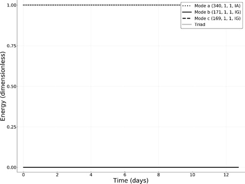
Fig. 4. Time evolution of the mode quadratic energies associated with the solution of the three-wave interaction equations (33)(33a) $$E_{a}A{\prime }_a={\sigma }_a^{bc}{A}_b{A}_c{e}^{-i{\delta }_{\mathit{abc}}t},$$(33a) for the modes of Triad 1 of Table 2. The present triad is nearly resonant.

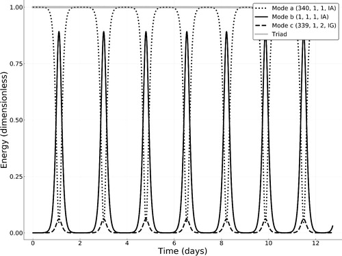
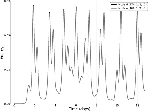
Fig. 5. Numerical solution of the linearized system (39) composed of modes (170,1,2,IG) and (169,1,2,IG) of Triad 2. These modes are parametrically forced by the mode (339, 1, 2, IG) of Triad 1. This solution presents a maximal Lyapunov exponent ${\lambda }_L=1.35\times {10}^{-5}{s}^{-1}.$

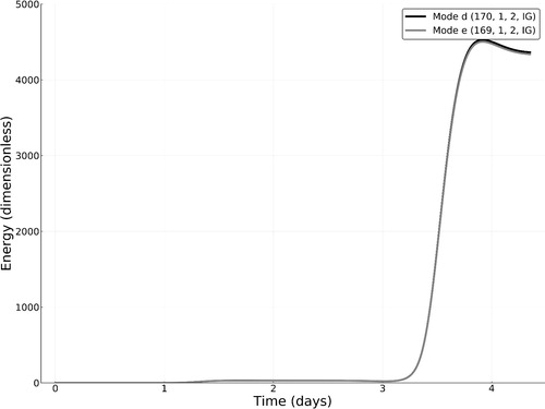
Fig. 6. Numerical solution of the linearized system (39) composed of modes (170,1,1,IG) and (169,1,1,IG) of Triad 13. These modes are parametrically forced by the mode (339, 1, 2, IG) of Triad 1. This solution presents a maximal Lyapunov exponent ${\lambda }_L=-4.85\times {10}^{-10}{s}^{-1}.$

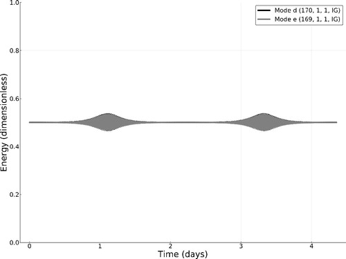
Fig. 7. Numerical solution of the linearized system (39) composed of modes (169,1,2,IG) and (–168,1,1,IG) of Triad 15. These modes are parametrically forced by the mode (1, 1, 1, IA) of Triad 1. This solution presents a maximal Lyapunov exponent ${\lambda }_L=6.59\times {10}^{-11}{s}^{-1}.$

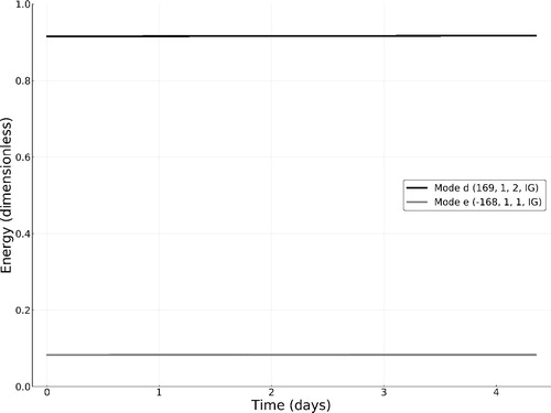
Fig. 8. Numerical solution of the five-wave system (38) composed of the modes of Triads 1 and 2 of Table 2. This figure illustrates the time evolution of the quadratic energies corresponding to Modes of Triad 1 only.

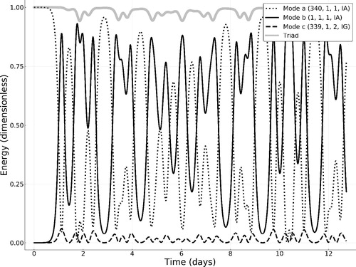
Fig. 9. This is same as Fig. 8, but illustrating the quadratic energies of the secondary gravity modes of Triad 2.