Impact of climate change on the climatology of Vb cyclones

Figures & data

Fig. 1. The CESM output and the three nested domains (D1 to D3) with the actual topography implemented in the simulations in metres above sea level are depicted. The horizontal resolutions of D1, D2 and D3 are 27, 9 and 3 km, respectively. In D1 the typical pathway of a Vb cyclone is shown as blue line. In D2 the origin (O), end (E) and restriction (R) boxes used to extract Vb cyclones are depicted as blue and violet boxes, respectively. The box labelled ‘Alps’ in D3 denotes the area used for calculating the precipitation intensity of the Vb events.

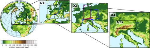
Fig. 2. Bootstrap probability density function of the accumulated precipitation from CESM data (1979–2013) in periods of time whose length mimics that of typical Vb events (black line) for extended summer (upper panel) and extended winter (lower panel). The red vertical lines indicate the 25th, 50th, 75th and 95th percentile from left to right. The vertical blue bars indicate the accumulated precipitation over the Alpine box (see Fig. 1 for the exact location of this box) of all the simulated Vb cyclones occurring during each season, respectively. The precipitation is obtained from the GCM directly.

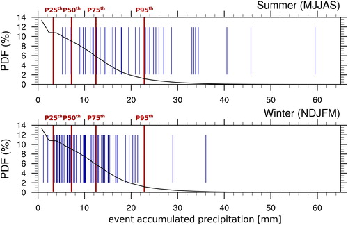
Fig. 3. Annual cyclone frequency of all detected cyclone centres (not only Vb cyclones) for the seamless CESM run and the period 1979–2013 (a), 2070–2099 (b) and the difference between (b) and (a) in (c). (d) and (e) show the annual cyclone frequency of all detected cyclones for the LENS for the period 1990–2005 and 2071–2080, respectively. (f) shows the difference between (e) and (d). The hatched area shows significant changes using a non-parametric Mann-Whitney-U test on a 10% and 5% level for (c) and (f), respectively. The grey area indicates places, where the topography exceeds 1000 meters above sea level.

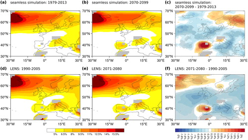
Fig. 4. Annual cyclone frequency of cyclones that pass through the origin box, labeled with ‘O’. The other two boxes indicate the end box (‘E’) and the restriction box (‘R’). (a) and (b) depict the frequency obtained from the seamless CESM run in the period 1979–2013 and 2070–2099, respectively. (c) shows the difference between (b) and (a). (d) and (e) illustrate the frequency of the LENS for the periods 1990–2005 and 2071–2080, respectively. (f) shows the difference between (e) and (d). The hatched area indicates significant changes on a 10% and 5% significance level, for (c) and (f), respectively, using the nonparametric Mann-Whitney-U test. The grey area indicates places, where the topography exceeds 1000 meters above sea level.

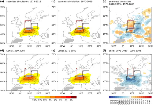
Fig. 5. The mean annual Vb cyclone frequency of the seamless CESM simulation for the period 1979–2013 (a) and 2070–2099 (b) and (c) showing the difference between (b) and (a). (d) and (e) show the same, but for the LENS and the period 1990–2005 and 2071–2080, respectively. (f) indicates the difference between (e) and (d). The hatched area indicates significant changes on a 10% and 5% significance level, for (c) and (f), respectively, using the nonparametric Mann-Whitney-U test. The grey area indicates places, where the topography exceeds 1000 meters above sea level.

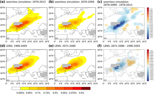
Fig. 6. (a) the mean annual number of Vb cyclones per month in the period between 1979–2013 (blue bars) and 2070–2099 (red bars) during the respective months (x-axis). (b) The distribution of the 10 heavy precipitation summer Vb events of both periods. (c) monthly average Mediterranean sea surface temperature (SST) and European 2-m temperature (2-m T) of the past period (blue lines) and the future period (red lines). The grey shaded area covers the months of the year that do not belong to the analysed extended summer season (MJJAS). (d) the mean monthly distribution of the 10 heavy precipitation summer Vb events found in the LENS for the periods 1990–2005 (blue bars) and 2071–2080 (red bars). The black lines indicate ± one standard deviation.

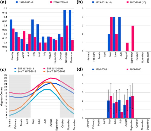
Fig. 7. Average daily precipitation of the 10 most intense precipitation summer Vb events for the CESM (left column) and WRF (right column) output for the period 1979–2013 (a and d) and 2070–2099 (b and e). (c) and (f) depict differences between (b) and (a) and (e) and (d), respectively. Shading indicates precipitation in mm day⁻¹. Hatched areas indicate significant changes using the non-parametric Mann-Whitney-U test and a significance level α = 10%.

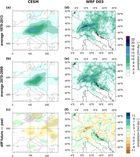
Fig. 8. The panels show the mean over 10 Vb events for the period between 1979–2013 (blue bar) and 2070–2099 (red bar). The depicted variables are (a) mean daily precipitation [mm], (b) mean daily upward moisture flux over land [kg m⁻²day⁻¹], (c) mean daily upward moisture flux over the ocean [kg m⁻²day⁻¹], (d) precipitable water [kg m⁻²], (e) mean daily precipitation over the Alps [mm], (f) mean daily sea surface temperature [° C], (g) mean daily air temperature at 850 hPa [° C], and (h) mean daily 2-m air temperature [° C]. All panels except for (e) show a spatial mean over domain 3, whereas (e) shows a spatial mean over the Alpine box. Asterisks located over the red bars indicate that the future values are significantly different from the past ones using the non-parametric Mann-Whitney-U test and a significance level α = 10%. The black vertical bar indicates ± one standard deviation across the 10 events.

Fig. 9. Average daily 2-m temperature of the 10 most intense precipitation summer Vb events for the domain 3 of the WRF simulations for the period 1979–2013 (a) and 2070–2099 (b). (c) depicts the differences between (b) and (a). Shading indicates the temperature in K. No statistical significance can be found on a 5% level.

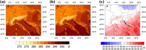
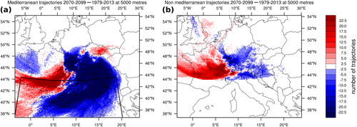
Fig. 10. Shading indicates the differences in the location of the 48-hour backward trajectories between averages of the 10 events of the period 2070–2099 and 1979–2013. Note that different trajectories can pass a certain point several times. The difference indicates a reduced or increased air parcel passage. The starting position is at 5000 m. (a) shows all the trajectories that pass through the Mediterranean region (black box), while (b) shows the trajectories that do not pass through the Mediterranean region.