Figures & data
Fig. 1. (a): ‘Natural color’ composite image of the Meteosat satellite (Source: NERC satellite receiving station, Dundee University) for 12 UTC, 24 April 2013. Clouds containing ice particles are colored in cyan. (b): Mean sea level pressure (contour) and near surface temperature from the ECMWF operational analysis with approximately 15 km horizontal resolution, providing the external forcing for the applied model chain. (c): Vertically-pointing range corrected backscatter signal at 820 nm wave length of the Hohenheim WVDIAL system.
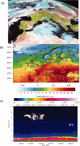
Fig. 2. Domain configuration of the WRF model chain. (a): Outer three domains with 2700 m resolution (D01), 900 m resolution (D02) and 300 m resolution (D03). (b): Domain 03 (300 m) including the inner domain with 100 m resolution.
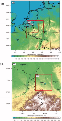
Fig. 3. Refinement of the representation of orography in the region of interest from 2700 m, 900 m, 300 m and 100 m. For the outer domain, the default data of the WRF pre-processing system (WPS) were used. The orography for the three inner domains were derived from the 90 m Shuttle Radar Topography Mission (SRTM) data set.
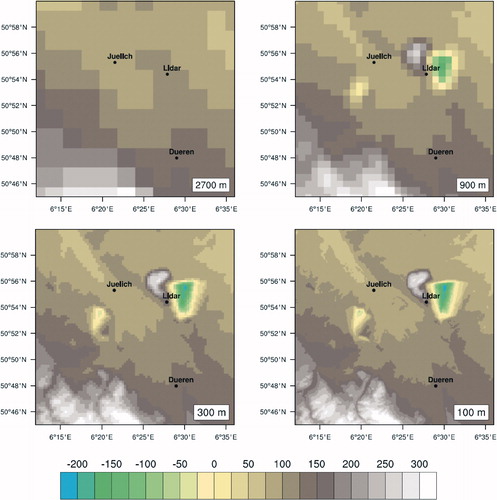
Fig. 4. Flow chart illustrating the setup of the model chain for the simulations.
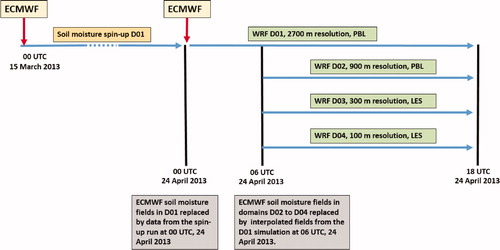
Fig. 5. Land use categories (100 m resolution) (a) and soil categories (1000 m resolution) (b) applied as lower boundary forcing for the WRF simulations.
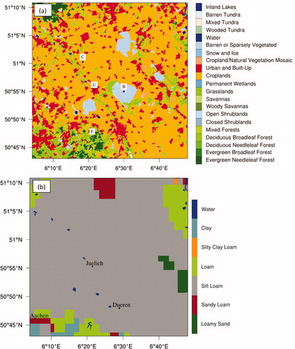
Table 1. Selected switches for the NOAHMP land surface model.
Table 2. Namelist configuration of the WRF-LES mode.
Fig. 6. Representation of vertical velocity 1000 m above sea level on April 24, 2013 at 13 UTC for four different model configurations. Shown is the innermost model domain with 100 m horizontal resolution. CTRL: 301 × 301 grid points with 57 vertical levels (15 in the boundary layer) and turbulence parameterization in the surrounding 300 m domain. EXP_A: As CTRL, but without turbulence parameterization in the 300 m domain. EXP_B: As EXP_A, but with 121 vertical levels (more than 30 in the boundary layer). EXP_C: As EXP_B, but with a larger domain size of 502 × 502 grid points. The green dot marks the location of the Hohenheim lidar systems.
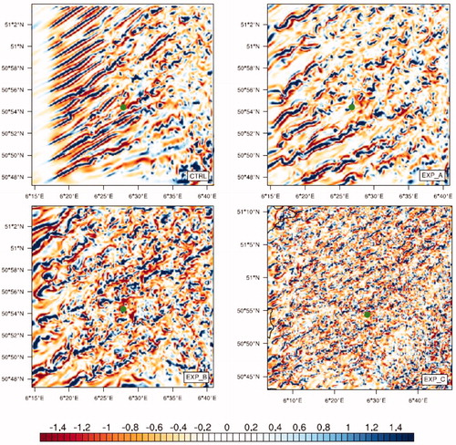
Table 3. Configuration of the different experiments to optimize the WRF-LES performance.
Fig. 7. Water vapor mixing ratio (g/kg) (panels a and c) and vertical velocity (m/s) (panels b and d) interpolated to 1000 m above sea level for 07 UTC (panels a and b) and 09 UTC (panels c and d), 24 April 2013.
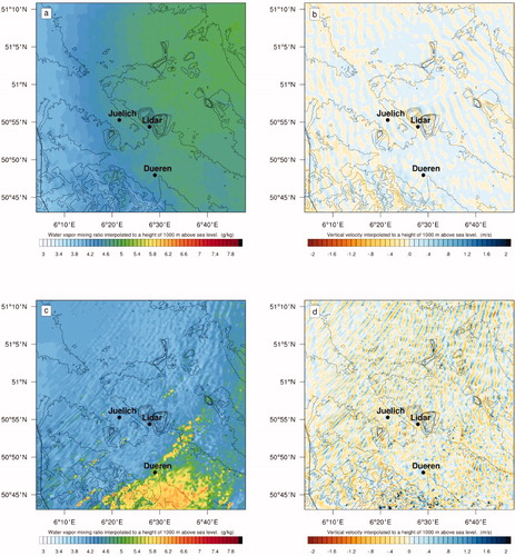
Fig. 8. Same as , but for 12 UTC (panels a and b) and 15 UTC (panels c and d), 24 April 2013.
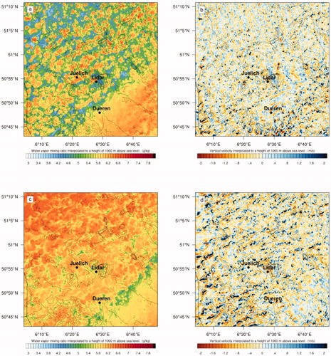
Fig. 9. Time-height cross sections of the lowest 1.8 km of the model atmosphere of simulated water vapor mixing ratio (g/kg) at the location of the Hohenheim lidar system (12 second averages calculated from the model time step output) for the period 06 to 18 UTC, 24 April 2013. From (a) to (d): 2700 m 900 m 300 m and 100 m horizontal resolution.
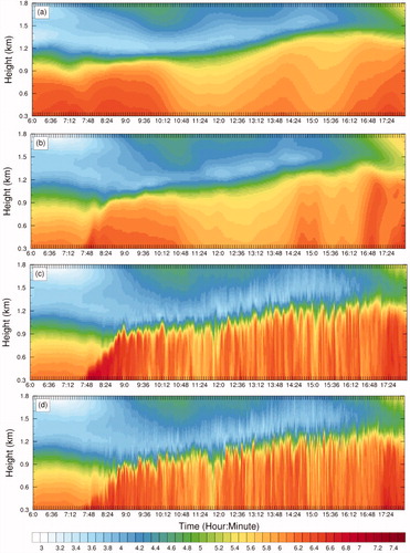
Fig. 10. Evolution of the boundary layer over different land cover classes as seen in time-height cross sections of simulated water vapor mixing ratio (g/kg). From (a) to (d), the underlying land cover classes are cropland, urban, barren/sparsely vegetated and forest. Results are shown from the innermost 100 m domain.
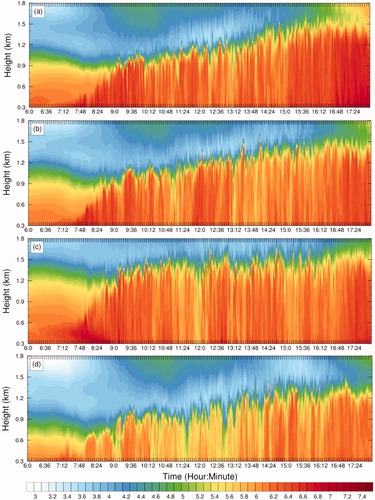
Fig. 11. Time-height cross sections of the lowest 1.8 km of the atmosphere of potential temperature (K). WRF simulation with 100 m resolution (a) and TRRL observation (b) for the period 12 to 14 UTC, 24 April 2013.
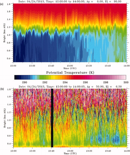
Fig. 12. Time-height cross sections of the lowest 1.8 km of the atmosphere of specific humidity (g/kg). WRF simulation with 100 m resolution (a) and WVDIAL observation (b) for the period 12 to 14 UTC, 24 April 2013.
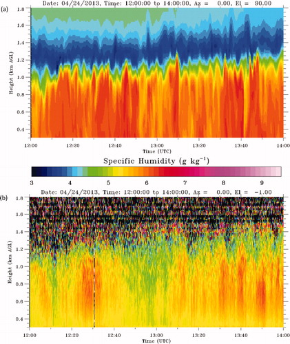
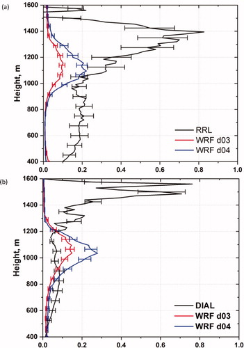
Fig. 13. Comparison of observed and simulated mean vertical profiles of potential temperature (K) (a) and specific humidity (g/kg) (b) for the period 12 to 14 UTC, 24 April 2013.
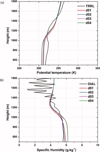
Table 4. Average PBL height for the observations and the different model resolutions during the period 12 to 14 UTC, 24 April 2013.
Fig. 14. Comparison of observed and simulated vertical profiles of temporal variances of potential temperature (K2) (a) and specific humidity (g2/kg2) (b) for the period 12 to 14 UTC, 24 April 2013.