Identifying remote sources of interannual variability for summer precipitation over Nordic European countries tied to global teleconnection wave patterns

Figures & data

Fig. 1. Pearson correlation between regionally averaged summer (JJA) precipitation over SwedFin and global z500 during (a) January, (b) February, (c) March, (d) April, (e) May, (f) June, (g) July and (h) August. Precipitation data from E-Obs and z500 from ERA5.

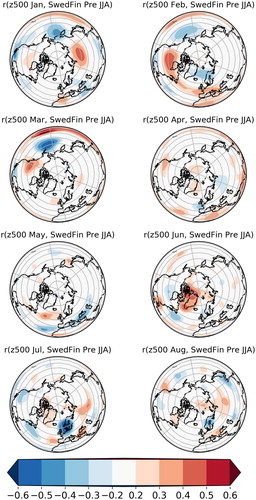
Fig. 2. (a) Pearson correlation between regionally averaged summer (JJA) precipitation over SwedFin and global z500 during March for every grid point. Regions of West of Hawaii (WH) and western Canada (WCan) that are used as predictors for summer precipitation are enclosed in yellow rectangles. (b) Standardized (removed the mean and divided by the standard deviation) time series of the PNA and of spatially averaged z500 over WH from ERA5. PNA data was downloaded from the webpage https://www.esrl.noaa.gov/psd/data/correlation/pna.data. Precipitation data from E-Obs.

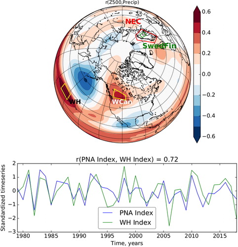
Fig. 3. Correlation between Niño3 index and geopotential height at 500 hPa. Enclosed are shown the WH and WCan regions used as z500-based predictors, which show some regions of coincidence with same sign correlation values as Figure 2a. NEC and SwedFin regions for summer precipitation are also shown. Niño3 index from https://psl.noaa.gov/gcos_wgsp/Timeseries/Data/nino3.long.anom.data. Z500 data from ERA5.

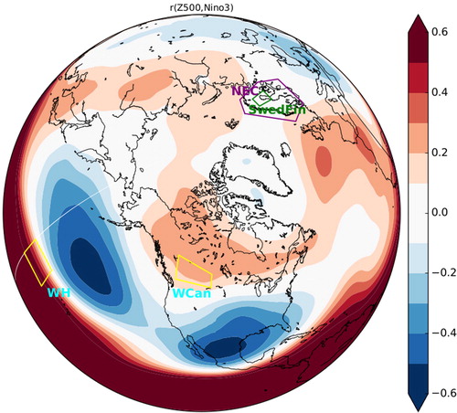
Fig. 4. Standardized time series of ENSO indices during March and summer (JJA) precipitation over NEC and SwedFin regions. The correlation coefficients between SwedFin precipitation and ENSO indices: r(SwedFin, Nino1 + 2) = 0.36, r(SwedFin, Nino3) = 0.36, r(SwedFin, Nino3.4) = 0.29, r(SwedFin, Nino4) = 0.10. Niño indices from https://psl.noaa.gov/gcos_wgsp/Timeseries/, precipitation from E-Obs.

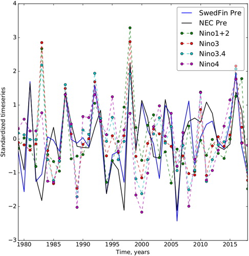
Fig. 5. Correlation between z500 during March averaged over WH with (a) omega (averaged along the tropical band between the latitudes 13 N-22 N) during summer, (b) vertically integrated moisture divergence (VIMD) during summer, (c) geopotential height at 500 hPa (z500) during summer, (d) two metre air temperature (Ts) during summer, (e) sea ice concentration during summer and (f) precipitation during summer. Correlation values abs(r) > 0.26 are statistically significant at p < 0.1. Omega, VIMD, z500 and Ts variables are from ERA5. Precipitation from E-Obs. Sea ice concentration from GLORYS2V4, and precipitation from E-Obs.

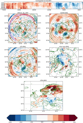
Fig. 6. Correlation between summer z500 and (a) CGT index, (b) SNAO, (c) SEA, (d) WH and WCan predictors based on z500 during March. All indices were calculated using ERA5 data.

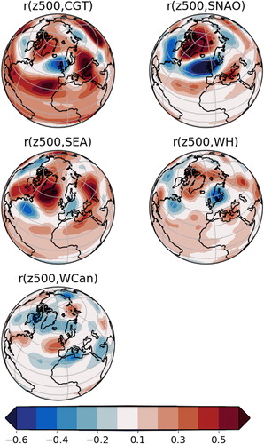
Fig. 7. Correlation between summer precipitation and (a) CGT index, (b) SNAO, (c) SEA, (d) WH and (e) WCan predictors based on z500 during March. Global precipitation from the Global Precipitation Climatology Project (GPCP) Monthly Analysis (New Version 2.3). z500 indices calculated with ERA5 data.

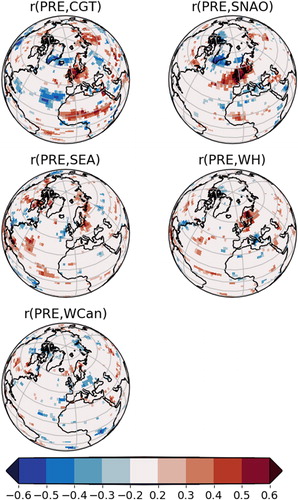
Fig. 8. (a) Time series of observed (E-obs) summer precipitation over the SwedFin region and time series of forecast precipitation from the leave-one-out cross-validation. (b) β₁ weights of predictor WH, (c) β₂ weights of predictor WCan, (d) correlation between summer observed precipitation and modelled precipitation, (e) HSS values for the modelled precipitation. HSS as described in Equation 1(1) $$\mathit{HSS}=\frac{\mathit{Hits}-L/3}{L-L/3}$$(1) is multiplied by 100%, (f) observed and (g) modelled precipitation anomaly in summer of 1981. (h) observed and (i) modelled precipitation anomaly in summer of 2018. The precipitation anomalies in (f)–(i) are shown in (wet, normal and dry) with standard deviations as units considering dry years when P < −0.5σ, normal when P is within ±0.5σ and wet with P > +0.5 σ.

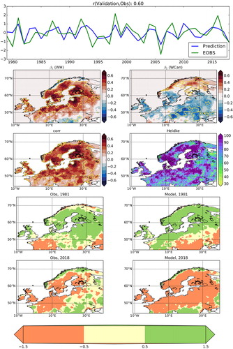
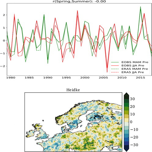
Fig. 9. Upper figure shows standardized precipitation time series over the SwedFin region for spring (MAM) and summer (JJA). Precipitation data from ERA5 and E-Obs. Lower figure shows HSS values for the spring precipitation anomalies as predictors for summer precipitation anomalies. HSS as described in Equation 1(1) $$\mathit{HSS}=\frac{\mathit{Hits}-L/3}{L-L/3}$$(1) is multiplied by 100%.