On the contribution of internal climate variability to European future climate trends

Figures & data

Table 1. Model simulations used for the analysis.

Ensemble	Time-period	Number of members
MPI-ESM-GE	1850–2100 Hist + RCP4.5	100
CanESM2-LENS	1950–2100 Hist + RCP8.5	50
CMIP5	1850–2100 Hist + RCP4.5 + RCP8.5	34 in total, 1 member per model: ACCESS1-0, ACCESS1-3, BCC-CSM1-1, CanESM2, CCSM4, CMCC-CM, CMCC-CMS, CNRM-CM5, CSIRO-Mk3-6-0, EC-EARTH, FGOALS-g2, FIO-ESM, GFDL-CM3, GFDL-ESM2G, GFDL-ESM2M, GISS-E2-H, GISS-E2-R-CC, GISS-E2-R, HadCM3, HadGEM2-AO, HadGEM2-CC, HadGEM2-ES, INMCM4_ESM, IPSL-CM5A-LR, IPSL-CM5A-MR, IPSL-CM5B-LR, MIROC5, MIROC-ESM-CHEM, MIROC-ESM, MPI-ESM-LR, MPI-ESM-MR, MRI-CGCM3, NorESM1-ME, NorESM1-M

Fig. 1. Winter (DJF average) and summer (JJA average) two-meter air temperature (T2m) trends in ERA-interim data (a, e), the ensemble means of MPI-ESM-GE (b, f), CanESM2-LENS (c, g) and CMIP5 (d, h) in the period 1985–2014. The lower row (i-l) shows the winter T2m trends in single ensemble members of MPI-ESM-GE and CanESM2-LENS. Shown are trends in Kelvin per 30 years. Note that the color-scale is not linear.

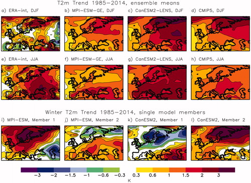
Fig. 2. As Fig. 1 but for precipitation. Shown are trends in mm/month per 30 years.

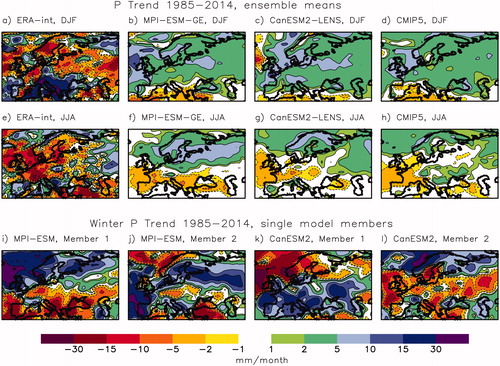
Fig. 3. Ensemble means of winter and summer two-meter air temperature trends (Kelvin per 30 years) in MPI-ESM-GE, CanESM2-LENS and CMIP5 (RCP4.5 and RCP8.5) between 2021 and 2050 (a–h) and their standard deviation across ensemble members (i–p). Note that the color-scale is not linear.

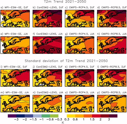
Fig. 4. As Fig. 3 but for precipitation.

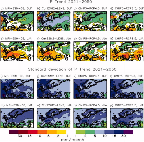
Fig. 5. As Fig. 3 but for the period 2021–2100. Shown are trends in Kelvin per 80 years.

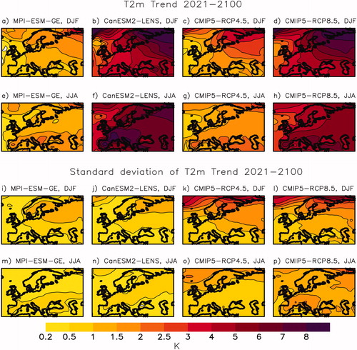
Fig. 6. Distribution of observed seasonal temperature trends over 30-year periods in Uppsala between 1722 and 2017 (number of cases per 0.5 K interval).

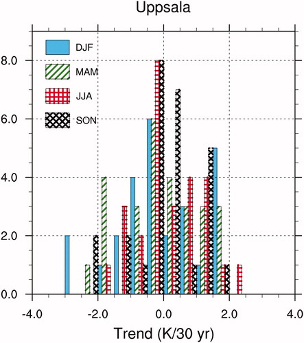
Fig. 7. Probability distribution of two-meter air temperature (top) and precipitation (bottom) trends in southern Sweden in winter (left) and summer (right) between 2021 and 2050. Shown are trends per 30 years. Intervals for temperature are 0.5K, for precipitation 5mm/month.

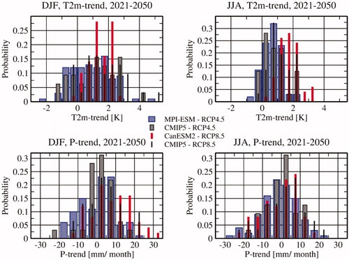
Fig. 8. Scatterplot of precipitation and two-meter temperature trends in southern Sweden in winter (left) and summer (right) in the period 2021–2050 in the MPI-ESM-GE (a-b) and CanESM2-LENS (c-d). Shown are trends per 30 years.

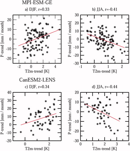
Fig. 9. Correlation between winter trends in T2m in southern Sweden in 2021–2050 and winter T2m trends in 2021–2050 (a and e), and winter sea level pressure (SLP) trends in 2021–2050 (b and f) in the MPI-ESM-GE (a–d) and CanESM2-LENS (e–h). (c, d, g and h) show the same as (a, b, e and f) but for summer T2m and SLP. Using a two-sided t-test, correlation coefficients above 0.2 and 0.29 are statistically significant at the 95% level assuming 100 degrees of freedom (MPI-ESM-GE,100 ensemble members) and 50 degrees of freedom (Can-ESM-LENS, 50 ensemble members), respectively.

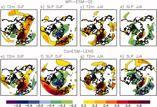
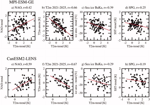
Fig. 10. Scatterplot of winter T2m-trends in southern Sweden in 2021–2050 in MPI-ESM-GE and CanESM2-LENS versus winter NAO-index trends (a and e), winter T2m-anomalies averaged over the first 5 years of the 2021–2050 year period (2021–2025, b and f), sea ice area trends in the Barents/Kara Seas in 2021-2050 (c and g), trends in the sea surface temperature (SST) of the subpolar gyre (SPG) in 2021–2050 (d and h).