Multi-year ocean thermal variability

Figures & data

Fig. 1. Bathymetry of the model (km) at 1 km intervals. As the deep ocean influences the thermal structure with increasing duration, the complex geometry of the topography can be dominant in the physics dividing the ocean into a large number of regionally distinct places. Compare to Sverdrup et al. (1942, Plate 1). Inset here and in other figures is a histogram of the plotted values.

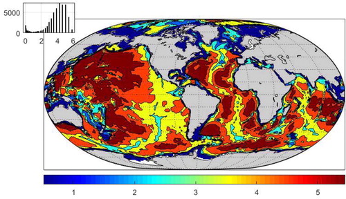
Fig. 2. Average potential temperature (not the anomaly) at 477 m during 1994. Note the multi-modality of the values (inset).

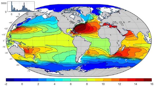
Fig. 3. Standard deviation (^oC) in time of annual mean temperature at 477 m over 26 years. Intricacy of the northern North Atlantic is apparent, as are the Kuroshio path, the region south of Cape Agulhas, and other ‘hot spots’. Spatial stationarity is an unattractive hypothesis.

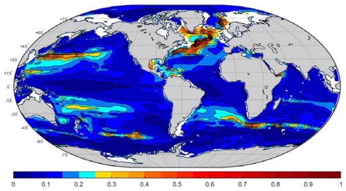
Fig. 4. Twenty-six year time-average of the vertical mean potential temperature (°C) in the ECCOv4r4 state estimate, ${\overline{T}}_G(\varphi ,\lambda ).$

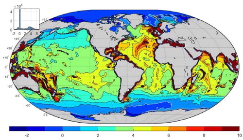
Fig. 5. Standard deviation (°C) for potential temperatures as a global average (a) and for the layer-thickness weighted values (b), m °C. Note use of the logarithmic scale for temperature alone. All model grid areas are given equal weight here.

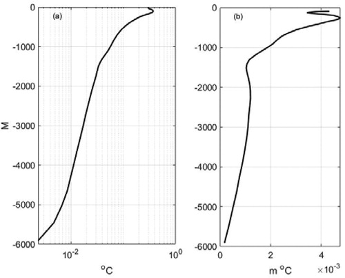
Fig. 6. Anomaly of vertically integrated temperature for 1993, $T_G(\lambda ,\varphi ,t=1993)$ (°C).

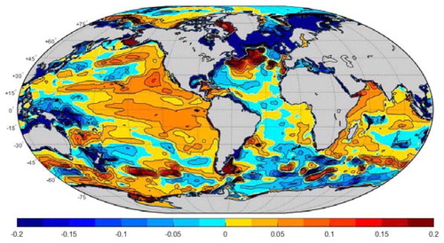
Fig. 7. Same as Fig. 6 except for 1998 – an El Niño year.

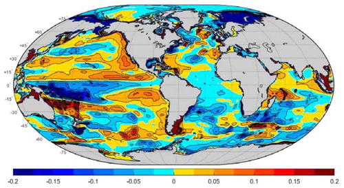
Fig. 8. Same as Fig. 6 except for 2017. An east-west basin divide occurs in the Atlantic Ocean.

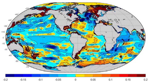
Table 1. Notation used when applying the SVD to differing fields. Singular vectors are all functions of a geographic coordinate, or of time.

SVD notation	Field	Dependence
${\mathbf{u}}_{rj,}{\lambda }_{rj},{\mathbf{v}}_{rj}$	Generic in space	Space coord., arbitrary field, arbitrary field
${\mathbf{u}}_{Tj,}{\lambda }_{Tj},{\mathbf{v}}_{Tj}$	Vertical temperature	Depth, temperature, time
${\mathbf{u}}_{dj,}{\lambda }_{dj},{\mathbf{v}}_{dj}$	Vertical thickness weighted	Depth, temperature × layer-thickness, time
${\mathbf{u}}_{Gj,}{\lambda }_{Gj},{\mathbf{v}}_{Gj}$	Global vert. avg. temperature	Latitude/longitude, Temperature, time

Fig. 9. (a) Global mean of first 3 vertical singular vectors. u ${}_{d1}(z)$ reaches 0.1 at a depth of 300 m and the plot is truncated for visibility. (b) Shows the accumulated variance in each global median ${\lambda }_{di}^2$ normalized to sum to 1. Roughly speaking, the lowest SVD carries about 75% of the variance and the first 3 represent over 95% of the variance. (c) Shows the first 3 ${\mathbf{v}}_{d1}(t).$

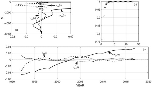
Fig. 10. The lowest singular vector ${\mathbf{u}}_{d1}$ at a variety of latitudes along 180° W (dimensionless). Greatest depths do not exist for these particular positions.

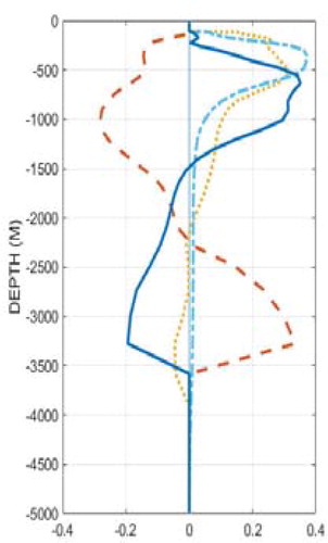
Fig. 11. (a) Fraction of the number of zeros occurring in all vertical modes ${\mathbf{u}}_d.$ (b) Fraction of the number of zeros occuring only in the lowest mode ${\mathbf{u}}_{d1}.$

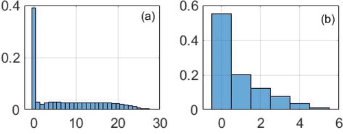
Fig. 12. Fraction of the vertical variance at each point in the lowest singular vector ${\mathbf{u}}_{d1}$ (dimensionless). It is, in general, not the same as a linear dynamical mode, but contains extra structure (zero crossings in the vertical).

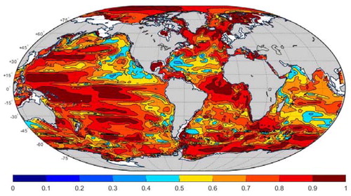
Fig. 13. (a) Global median singular values λ_Gj (°C) and their normalized cumulative sum (b). (c) Shows the mean temporal coefficients ${\mathbf{v}}_{Gj}(t)$ for $j=1,2,3.$

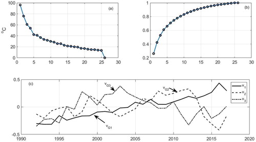
Fig. 14. Structure of 1000${\mathbf{u}}_{G1}$ mapped onto latitude and longitude (dimensionless). Sign change coincides with the yellow-blue boundary.

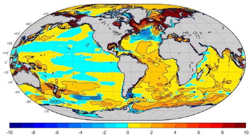
Fig. 15. $1000u_{G2}$ mapped onto latitude and longitude.

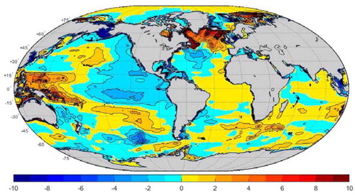
Fig. 16. 1000${\mathbf{u}}_{G3}.$ Western tropical Pacific and high North Atlantic structures are notable.

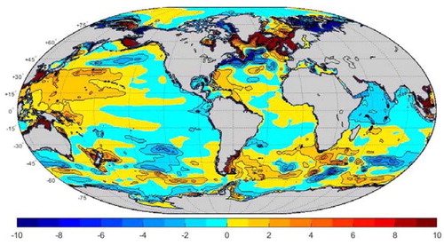
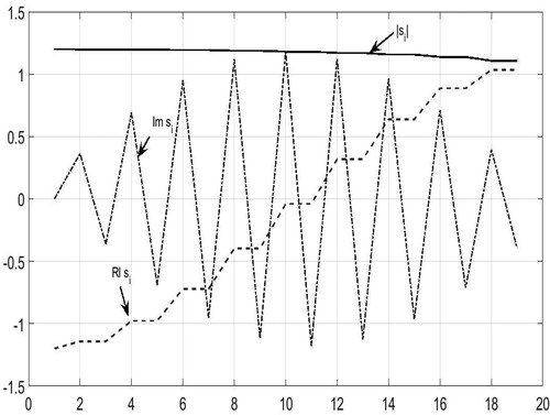
Fig. 17. Eigenvalues of the principal observation patterns (POPs), plotted as absolute value, real and imaginary parts.

Sverdrup, H. U., Johnson, M. W. and Fleming, R. H. 1942. The Oceans, Their Physics, Chemistry, and General Biology. Prentice-Hall, Inc., New York, 1087 pp.

 Google Scholar