Dynamically weighted hybrid gain data assimilation: perfect model testing

Figures & data

Fig. 1. Spatial distribution of synthetic observations.

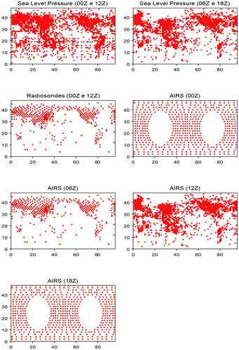
Fig. 2. Time-series (assimilation cycles) of root mean square error (RMSE), in red, and ensemble spread (SPRD), in blue, of Lorenz-96 analysis (top panel) and forecasts (bottom panel).

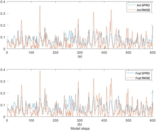
Fig. 3. Lorenz-96 LETKF analysis spread (SPRD) indexed by analysis error (RMSE) sorted from low to high values. Linear regression lines (dashed lines) show the small and steep growth rate of analysis spread as a function of analysis error growth (top panel). The spread–error relationship in the forecasts (bottom panel) shows similar results compared to the analysis error–spread relationship.

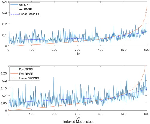
Fig. 4. Horizontal structure of the dynamic alpha (top) and spread (bottom) of the sea level pressure (ps) on February 28 at 18Z.

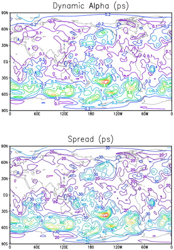
Fig. 5. Vertical structure of the dynamic alpha (top) and spread (bottom) of temperature (T) at the latitude 45°S on February 28 at 18Z.

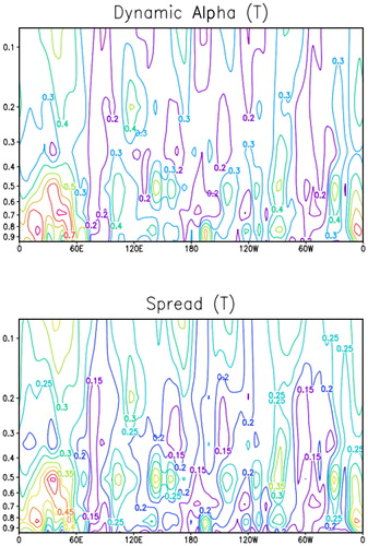
Fig. 6. Mean (top) and standard deviation (bottom) of alpha of the sea level pressure for the entire period of this study (December, January and February).

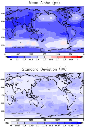
Table 1. Mean RMSE of pressure (ps), temperature (T) and wind components (u and v) over the globe in seven levels of the model.

	ps		T		u		v
	EKF	VAR	EKF	VAR	EKF	VAR	EKF	VAR
1	28.5	45.8	0.13	0.20	0.40	0.67	0.40	0.71
2			0.15	0.24	0.42	0.73	0.40	0.74
3			0.17	0.28	0.46	0.80	0.44	0.82
4			0.23	0.36	0.61	1.08	0.60	1.13
5			0.24	0.38	0.80	1.46	0.83	1.54
6			0.26	0.42	0.81	1.66	0.83	1.66
7			0.27	0.47	0.36	0.78	0.36	0.83

Fig. 7. Mean absolute wind error (500 hPa) in m/s for the eight experiments: dynamic alpha, $\alpha =0.1,\alpha =0.3,\alpha =0.5,\alpha =0.7,\alpha =0.9,$ LETKF and 3D-Var for the (red) Southern Hemisphere and (blue) Northern Hemisphere.

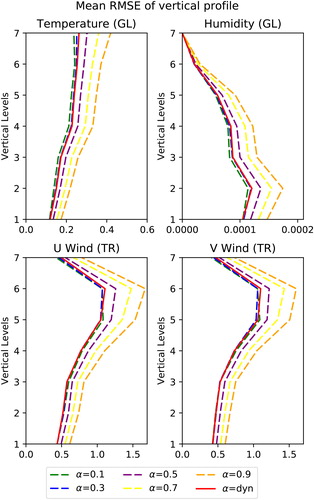
Fig. 8. Mean of ageostrophic wind (500 hPa) in m/s for the eight experiments: dynamic alpha, $\alpha =0.1,\alpha =0.3,\alpha =0.5,\alpha =0.7,\alpha =0.9,$ LETKF and 3D-Var for the (top) Northern Hemisphere and (bottom) Southern Hemisphere. The blue points are the experiment values, and the red lines indicate the values for the nature run.

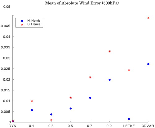
Fig. 9. Mean of ageostrophic wind (500 hPa) in m/s for the eight experiments: dynamic alpha, $\alpha =0.1,\alpha =0.3,\alpha =0.5,\alpha =0.7,\alpha =0.9,$ LETKF and 3D-Var for the (top) Northern Hemisphere and (bottom) Southern Hemisphere. The blue points are the experiment values, and the red lines indicate the values for the nature run.

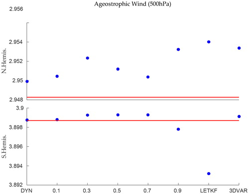
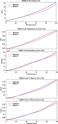
Fig. 10. RMSE of temperature, humidity, wind components (u and v) at level 4 and sea level pressure over the globe during the 120 h of forecast. The dynamic alpha experiment and experiment using α = 0.1 are shown as the red and blue lines, respectively.