Adding CO₂ channel 16 to AHI data assimilation over land further improves short-range rainfall forecasts

Figures & data

Fig. 1. Spatial distributions of the 24-h accumulative rainfall observations and geopotential height at 500 hPa (a) from 0000 UTC July 1 to 0000 UTC July 2 (case 1), (b) from 0000 UTC July 10 to 0000 UTC July 11 (case 2), and (c) from 1200 UTC July 19 to 1200 UTC July 20, 2016 (case 3).

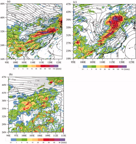
Fig. 2. Spatial distributions of 500-hPa geopotential height from the NCEP reanalysis (black curve, contour interval: 20 m) and relative humidity (color shading, unit: %) in the model domain at (a) 1200 UTC 18 July (beginning time of the DA cycling for case 3) and (b) 1200 UTC 19 July (ending time of the DA cycling for case 3), 2016.

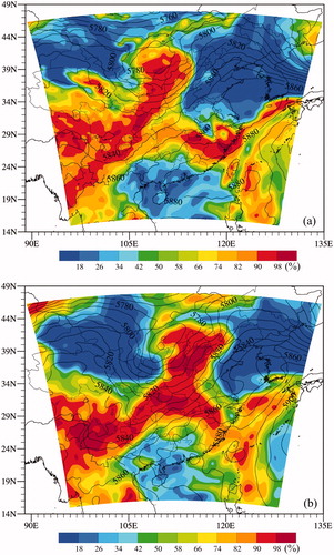
Fig. 3. (a) Mean (bars) and standard deviation (curves) of O-B for AHI channels 7–10 and 11–16 data over land (solid bars and open circles) and ocean (dashed bars and stars) calculated from all data from July 1 to 31, 2016 in the model domain. (b) Standard deviation of O-B varying with terrain height for AHI channels 7–10 and 11–16 calculated from all data from July 1 to 31, 2016 in the model domain.

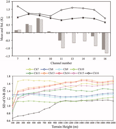
Fig. 4. (a) The mean (curve and open circle) and the one standard deviation (vertical line) of relative sensitivity of channel-16 brightness temperature to air temperature (curve) and surface emissivity (open circle) averaged for all data from July 1 to 31, 2016 in the model domain. (b) The mean (bars) and the one standard deviation (vertical lines) of maximum relative sensitivities of air temperature (solid bars) and surface emissivity (dashed bars) over meadow grass, barren soil and pine forest.

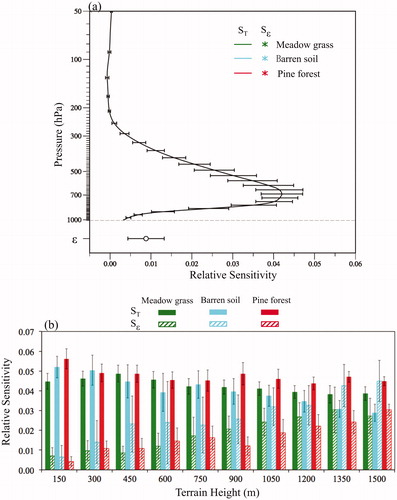
Fig. 5. Spatial distribution of the major surface types within 0.5 × 0.5 horizontal grid boxes (>50%) from NPOESS dataset, including water (blue), barren soil (barren, cyan), meadow grass (grass, green), grass shrub land (scrub, light green), irrigated low vegetation (lwbeg, yellow), boardleaf pine forest (bpforest, light orange), boardleaf forest (bforest, orange), pine forest (pforest, red), and mixed (grey, not a single surface exceeds 50%). Asterisks show the spatial locations of three selected data points used below.

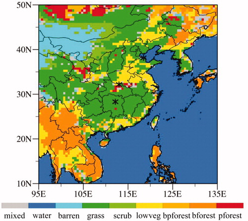
Fig. 6. (a) Vertical profiles of air temperature (solid curve) and specific humidity (dashed curve) and (b) relative sensitivity of channel-16 brightness temperature to air temperature (solid curve) and surface emissivity (stars) for the three land data points indicated in Fig. 5a (i.e. meadow grass, green; barren soil, cyan; and pine forest, red) at 1200 UTC 18 July 2016. Surface temperature at the meadow grass, barren soil, and pine forest points is 301.8, 300.19 and 303.26 K, respectively.

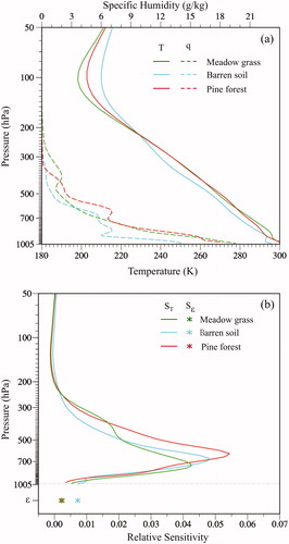
Fig. 7. Same as Fig. 6b except for (a) AHI channel 11 (solid curve and star) and 12 (dashed curve and open circle), (b) channel 13 (solid curve and star) and 14 (dashed curve and open circle).

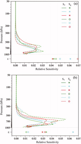
Fig. 8. Relative sensitivities of brightness temperatures for AHI channels 8 (green), 9 (blue), 10 (red) and 16 (black) to air temperature (solid curve), specific humidity (dashed curve) and surface emissivity (star) at 1200 UTC 18 July 2016 at (a) the pine forest point and (b) the broadleaf point indicated in Fig. 5a.

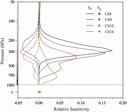
Fig. 9. Spatial distributions of O-B (left panels) and O-A (right panels) for (a)-(b) AHI channel 10 and (c)-(d) channel 16 at 0000 UTC 19 July 2016 for the experiment E4CH. Black dots represent data rejected by quality control. Black and white shaded represents the brightness temperature of AHI channel 14. The Magenta line shows the Tibet Plateau.

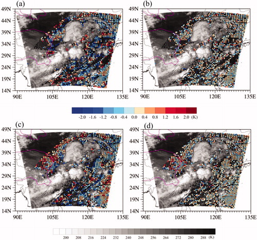
Fig. 10. Spatial distributions of the 500-hPa (a)-(b) geopotential height, (c)-(d) temperature and (e)-(f) specific humidity analyses from E4CH (left panels) and E3CH (right panels) (black curve) and the corresponding differences between E4CH and CONV (left panels) and those between E3CH and CONV (right panels) (color shading) at 0600 UTC 19 July 2016. The magenta curve shows the 2-km terrain height of the Tibet Plateau. The position of the cross sections in Fig. 11 is indicated in Fig. 10a.

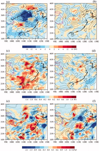
Fig. 11. Cross sections of the analysis differences of temperature (color shading), geopotential height (black contours at interval: 4 m), and wind (black arrow) between E4CH and E3CH (E4CH-E3CH) along the black dashed line in Fig. 10a at 1800 UTC 18 July, 0000, 0600, 1200 UTC 19 July 2016. Grey shaded areas represent the terrain height indicated by the y-axis on the right.

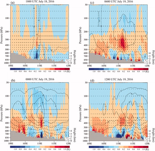
Fig. 12. Spatial distributions of (a) the 3-h accumulative rainfall observations during 0300–0600 UTC 20 July 2016, and the 15–18 h model forecasted rainfall amounts by (b) CONV, (c) E4CH and (d) E3CH.

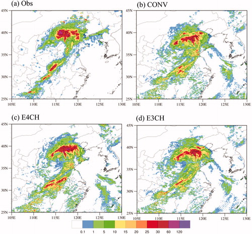
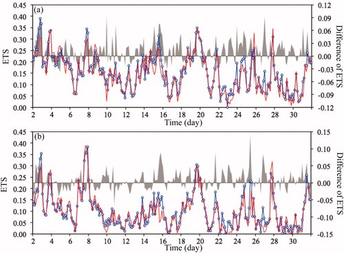
Fig. 14. Time series of the 3-h ETS for the E3CH (red) and E4CH (blue) experiments at the (a) 1-, (b) 5-mm thresholds during 2–31 July, 2016. The grey shading represents ETS differences between the two experiments (E4CH-E3CH) on every 3-h.