Some quantitative characteristics of error covariance for Kalman filters

Figures & data

Fig. 1. Examples of Kalman filter error covariance.

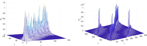
Fig. 2. A partition of error covariance.

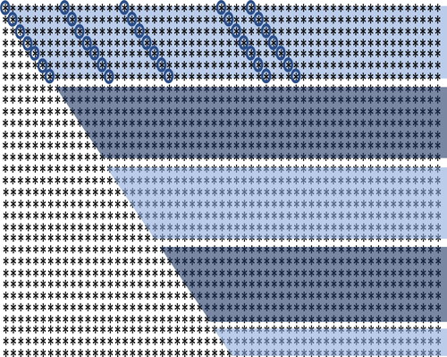
Fig. 3. Rows and columns of error covariance constrained by the observation model.

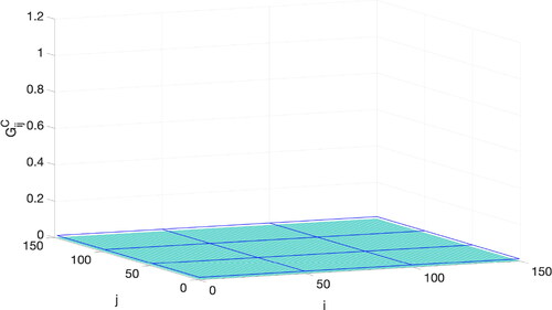
Fig. 4. The approximate peak value of error covariance computed using an upper bound matrix.

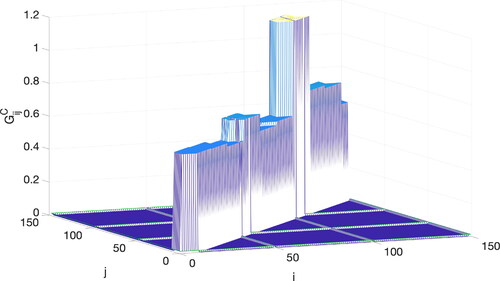
Fig. 5. The approximated shape (left) and the matrix upper bound (right) of the error covariance.

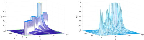
Fig. 6. The averaged error covariance along diagonals of blocks. The horizontal axis represents the indices of diagonals, where the middle point is the main diagonal. The vertical axis represents the average value of the elements in the error covariance along diagonals. The blue curve represents the true error covariance of a linear Kalman filter. The red curve is the matrix upper bound of error covariance. The green curve represents the approximated decay function.

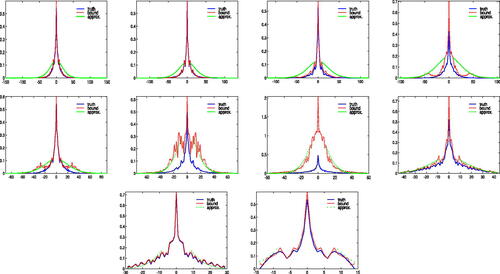
Fig. 7. The averaged error covariance along diagonals of two representative blocks. See the caption of Figure 6 for details.

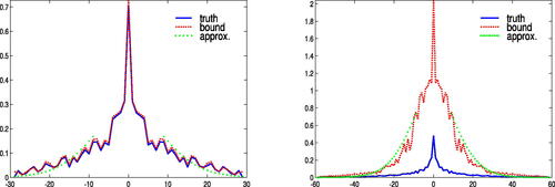
Fig. 8. Correlation functions.

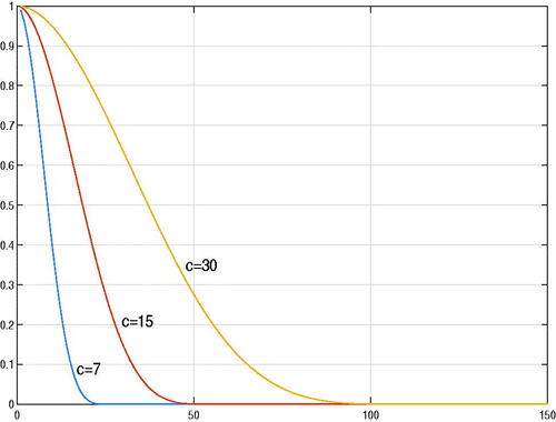
Fig. 9. The averaged error covariance along diagonals of blocks for localisation c = 30. The horizontal axis represents the indices of diagonals, where the middle point is the main diagonal. The vertical axis represents the average value of the elements of error covariance along diagonals. The blue curve represents the error covariance of an EnKF. The red curve is the matrix upper bound of error covariance. The green curve represents the approximated decay function.

Fig. 10. The state $x_1(t_f),x_2(t_f),\dots ,x_n(t_f)$ where n = 150. Solid: truth. Dotted: estimated value.

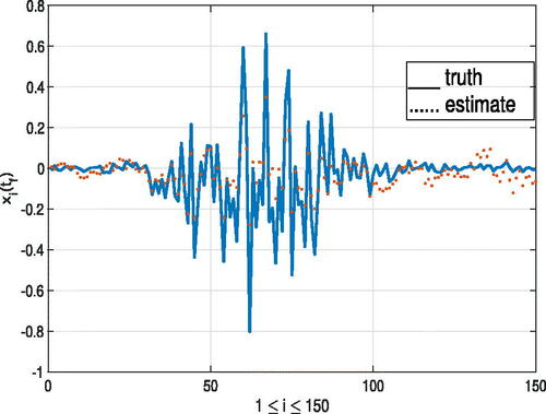
Fig. 11. The averaged error covariance along diagonals of blocks for localisation c = 7. See the caption of Figure 9 for details.

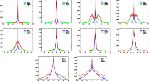
Fig. 12. The state $x_1(t_f),x_2(t_f),\dots ,x_n(t_f)$ where n = 150. Solid: truth. Dotted: estimated value.

Fig. 13. The variables in the model of a tsunami wave.

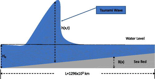
Table 1. The parameters in Example 3.

Parameter	L	T	H0	g
Value	$1,296\times {10}^3$ m	60,000 s	61.5m	9.81 m/s^2

Fig. 14. Water wave at t = 20,000, 40,000, 60,000 s.

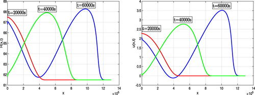
Fig. 15. UKF error covariance (the portion $1\le i,j\le 500$).

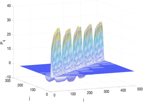
Fig. 16. UKF estimation at t = 60,000 s. Solid: truth. Dotted: estimated value.

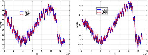
Fig. 17. The averaged error covariance along diagonals of the block between the rows $2001\le i\le 2100.$ See the caption of Figure 6 for details.

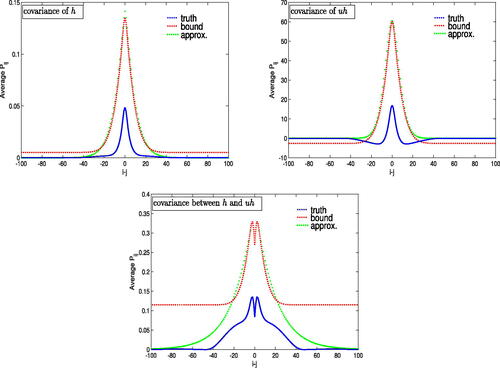
Fig. 18. The upper bound of error covariance deduced from observation model.

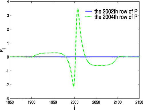
Fig. 19. Error covariance along two adjacent rows, i = 2002 and i = 2004.