An anisotropic formulation of the parametric Kalman filter assimilation

Figures & data

Fig. 1. Analysis-error aspect tensor fields for both PKF O2 (black ellipses) and PKF O1 (yellow ellipses): an observation placed at the centre (red dot) is assimilated with an observation error standard deviation of ${\sigma }^o=1.0$ in panel (a) and ${\sigma }^o=0.5$ in panel (b). One in five ellipses is shown here with a zoom on the centre of the domain and a scaling of 0.5 for the ellipse representation. The isotropy deviation ${\delta }_{\text{iso}}$ computed for PKF O2 is superimposed on the fields (the grey shading).

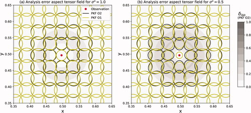
Fig. 2. Illustration of the non-divergent velocity field (a) whose integration from 0 to 3 has been used to transforms an isotropic aspect tensor field into an anisotropic one taken as the forecast error aspect tensor field. The ellipses in panel (b) and (c) show some of the forecast error aspect tensors, superimposed with the diagnosis of the deviations from isotropy (b) (0 indicates an isotropic tensor and 1 indicates a purely anisotropic tensor) and the isotropic length scale normalized by the grid spacing (c). The ellipses in the two panels (b) and (c), are the same, and the panels differ only by the shading.

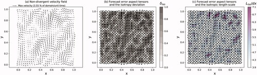
Fig. 3. Prescribed forecast-error correlation functions as specified from a diffusion formulation (a), and the heterogeneous Gaussian correlations (b), and defined from the aspect tensor field Fig. 2. The level sets of the iso-correlations $\{0.5,0.7,0.9\}$ are represented from light to dark grey.

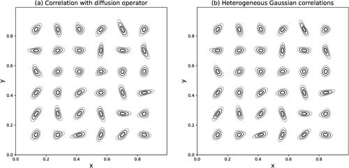
Fig. 4. The (a) true ${\mathcal{X}}^t$ and (b) forecast ${\mathcal{X}}^f$ states considered in the experiment with the observational network (the red dots in panel (a)) of 80 observed positions.

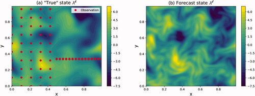
Fig. 5. Analysis increments for (a) the KF, (b) PKF O1 and (c) PKF O2.

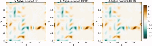
Table 1. Relative error for the analysis increment and error statistics with the KF as the reference.

PKF	$\frac{\left|\right|\delta {\mathcal{X}}^a(.)-\delta {\mathcal{X}}^a(KF)\left|\right|}{\left|\right|\delta {\mathcal{X}}^a(KF)\left|\right|}$	$\frac{\left|\right|V^a(.)-V^a(KF)\left|\right|}{\left|\right|V^a(KF)\left|\right|}$	$\frac{\sum _{\mathit{x}}\left|\right|{\mathbf{s}}_{\mathit{x}}^a(.)-{\mathbf{s}}_{\mathit{x}}^a(KF)\left|\right|}{\sum _{\mathit{x}}\left|\right|{\mathbf{s}}_{\mathit{x}}^a(KF)\left|\right|}$
O1	8.91%	1.26%	9.14%
O2	9.35%	1.01%	8.86%

$\left|\right|·\left|\right|$ stands for the L² norm. The results have been approximated to the hundredth of a percent.

Fig. 6. Analysis-error variance fields for the KF (a), the PKF O1 (b), and the PKF O2 (c).

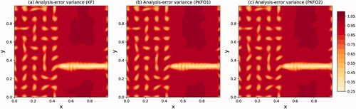
Fig. 7. Relative variation of the isotropic length scale, $r_{\text{iso}}^{af}=\frac{L_{\text{iso}}^a-L_{\text{iso}}^f}{L_{\text{iso}}^f},$ for the KF (a), the PKF O1 (b), and the PKF O2 (c). The white colour indicates values larger than those within the colour range.

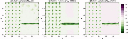
Fig. 8. Analysis increments resulting from the assimilation cycles using an EnKF of 1000 members (left column), the PKF O1 (middle column) and the PKF O2 (right column). Only the results at time 0 (top line), 3.5 (middle line) and 9 (bottom line) are shown, while an assimilation is performed each $\Delta t=0.5$ which represents 19 assimilation cycles. PKF O2 fails after $t=4.$

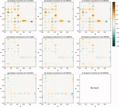
Fig. 9. Same as for Fig. 8 but for the analysis-error variance fields. In panel (a), the white colour indicates values larger than those of the colour range.

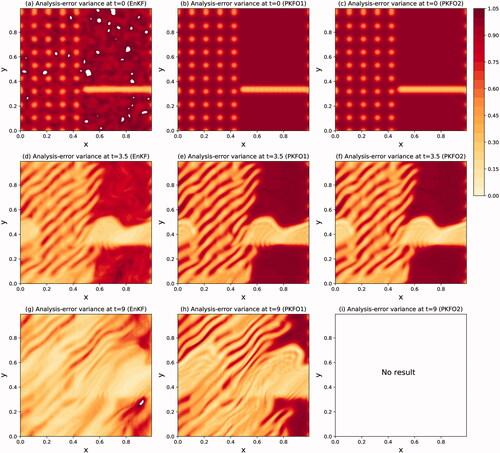
Fig. 10. Same as for Fig. 8 but for the relative variation of the isotropic analysis-error length-scale with respect to the initial isotropic length-scale $L_h=4\delta x,r_{\mathit{iso}}^{ah}=\frac{L_{\text{iso}}^a-L_h}{L_h}.$

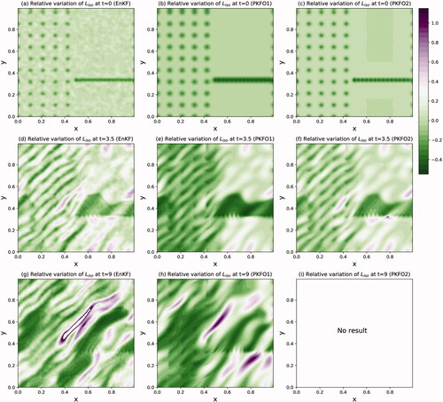
Fig. 11. Relative error of the EnKF and of the PKF O2 vs. the PKF O1 solution computed for the analysis state (a), the analysis-error variance field (b) and the analysis-error isotropic length-scale field (c). An assimilation is performed each $\Delta t=0.5.$

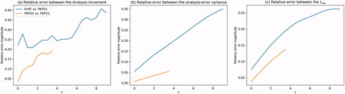
Fig. 12. Forecast-error variance (a) and relative isotropic length-scale (b) resulting from an ensemble of 1000 forecasts, integrated from time 0 to 9 without assimilation.

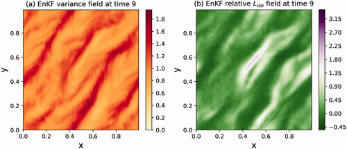
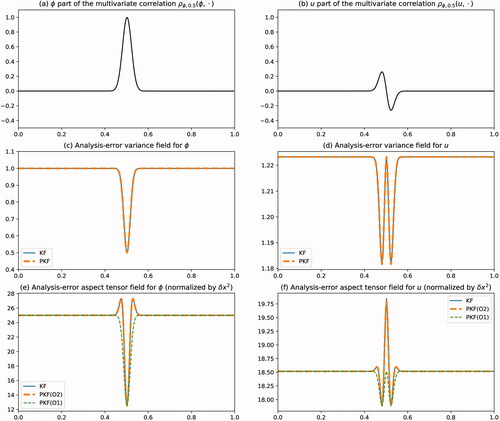
Fig. 13. Assimilation experiment of a single observation of $\varphi$ at x = 0.5. The multivariate correlation ${\rho }_{\varphi ,0.5}$ is shown in (a) and (b). The analysis-error variance fields are shown in (c) and (d) for the KF and the PKF computed from the multivariate Algorithm 2 and normalized by the initial forecast-error variance ($V^f{}_{\varphi }$ and $V^f{}_u$). The aspect tensor are shown in (e) and (f) for the KF, the PKFO2 and the PKFO1, and normalized by the initial forecast-error aspect tensor (${\mathit{s}}_{\varphi }^f$ and ${\mathit{s}}_u^f$).