1,662
Views
9
CrossRef citations to date
0
Altmetric
Articles

A decadal inversion of CO2 using the Global Eulerian–Lagrangian Coupled Atmospheric model (GELCA): sensitivity to the ground-based observation network

, , , , , , , , , & show all
Article: 1291158 | Received 28 Dec 2015, Accepted 29 Nov 2016, Published online: 03 Apr 2017

Figures & data

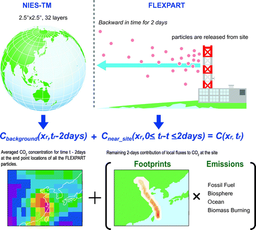
Fig. 1. Schematic diagram of GELCA inverse modelling framework.

Fig. 1. Schematic diagram of GELCA inverse modelling framework.

Fig. 2. Illustration of the inversion process employed in this study. The t indicates the time step on monthly basis. The modelled CO2 concentrations zmod are sum of the background concentrations zb and the presubtracted concentrations zp calculated by GELCA. In each inversion cycle, the modelled concentrations are compared to observations zob and the state vector s is optimized within a 3-month window. Optimized fluxes are incorporated into the background concentration () before calculating for the next time step. The number of asterisks in the upper right of s shows how many times a set of monthly fluxes has been optimized previously from past cycles. The prime in the upper right of zb means that the zb has been updated. The dashed arrows mean monthly calculations by GELCA.
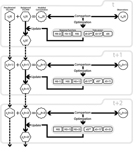
Fig. 2. Illustration of the inversion process employed in this study. The t indicates the time step on monthly basis. The modelled CO2 concentrations zmod are sum of the background concentrations zb and the presubtracted concentrations zp calculated by GELCA. In each inversion cycle, the modelled concentrations are compared to observations zob and the state vector s is optimized within a 3-month window. Optimized fluxes are incorporated into the background concentration () before calculating for the next time step. The number of asterisks in the upper right of s shows how many times a set of monthly fluxes has been optimized previously from past cycles. The prime in the upper right of zb means that the zb has been updated. The dashed arrows mean monthly calculations by GELCA.

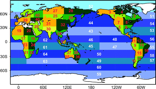
Fig. 3. Definitions of the 64 regions used in the inversion.

Fig. 3. Definitions of the 64 regions used in the inversion.

Table 1. Observational sites used in this study, including the model–data mismatch results for the control case inversion. Check marks in the last four columns show whether the site is used in the indicated case.

Table 2. Types of observation sites used in each case.

Fig. 4. Map showing the observation site locations of the different site selection cases: (a) control case (all symbols), Case SEL (green symbols removed), and Case NA (red symbols removed); (b) Case CT and (c) Case NF. Symbol shapes indicate the type of sampling: ○, surface discrete; +, surface continuous; ▾, ship; ♢, aircraft.
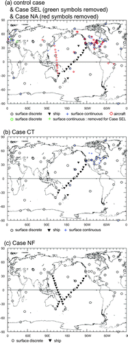
Fig. 4. Map showing the observation site locations of the different site selection cases: (a) control case (all symbols), Case SEL (green symbols removed), and Case NA (red symbols removed); (b) Case CT and (c) Case NF. Symbol shapes indicate the type of sampling: ○, surface discrete; +, surface continuous; ▾, ship; ♢, aircraft.

Fig. 5. Comparison of global annual mean posterior fluxes: (a) net, (b) land biosphere, and (c) ocean. (d) Multivariate ENSO Index (MEI) (Wolter and Timlin, Citation1993) for 2002–2011. Positive fluxes indicate emission and negative fluxes indicate uptake. In (a), the global annual mean atmospheric CO2 growth rate is shown with net fluxes. The CO2 growth rate in ppm are converted to the emission rates in Pg of carbon with a conversion factor of 2.12 PgC ppm−1 via simple molecular weight considerations. In (b) and (c), the global annual mean prior fluxes for land biosphere and ocean are shown, respectively.
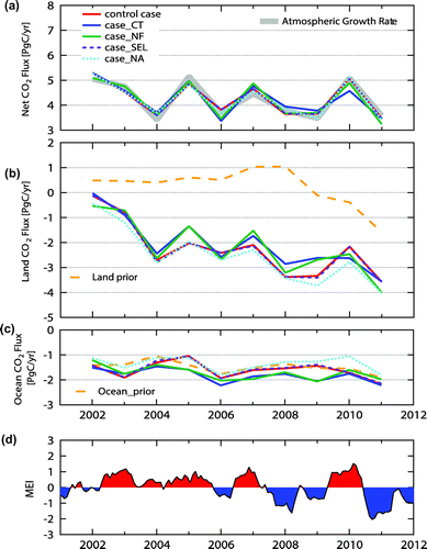
Fig. 5. Comparison of global annual mean posterior fluxes: (a) net, (b) land biosphere, and (c) ocean. (d) Multivariate ENSO Index (MEI) (Wolter and Timlin, Citation1993) for 2002–2011. Positive fluxes indicate emission and negative fluxes indicate uptake. In (a), the global annual mean atmospheric CO2 growth rate is shown with net fluxes. The CO2 growth rate in ppm are converted to the emission rates in Pg of carbon with a conversion factor of 2.12 PgC ppm−1 via simple molecular weight considerations. In (b) and (c), the global annual mean prior fluxes for land biosphere and ocean are shown, respectively.

Fig. 6. Decadal mean (2002–11) spatial distributions of posterior fluxes for (a–c) land and (e–g) ocean regions: (a, e) control case, (b, f) Case CT, (c, g) Case NF. Prior fluxes from the (d) land biosphere and (h) ocean. Positive fluxes indicate emission and negative fluxes indicate uptake.
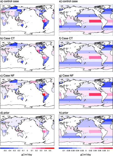
Fig. 6. Decadal mean (2002–11) spatial distributions of posterior fluxes for (a–c) land and (e–g) ocean regions: (a, e) control case, (b, f) Case CT, (c, g) Case NF. Prior fluxes from the (d) land biosphere and (h) ocean. Positive fluxes indicate emission and negative fluxes indicate uptake.

Table 3. The number of data used in the inversion, mean bias, root-mean-square error (RMSE), and correlation coefficient (R): (a) control case, Case CT, and Case NF; and (b) control case, Case SEL, and Case NA.

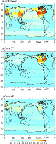
Fig. 7. Uncertainty reductions by region: (a) control case, (b) Case CT, and (c) Case NF.

Fig. 7. Uncertainty reductions by region: (a) control case, (b) Case CT, and (c) Case NF.

Fig. 8. Model–data mismatch for observation sites after inversion: (a) control case, (b) Case CT, (c) Case NF. The colour and size of the coloured circles indicate the bias and the RMSE, respectively. The size of the open circles indicates the prior uncertainty value.
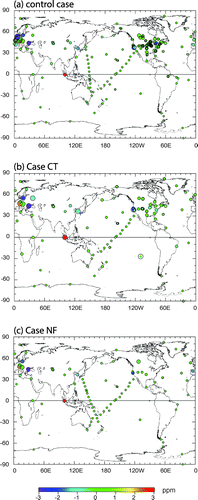
Fig. 8. Model–data mismatch for observation sites after inversion: (a) control case, (b) Case CT, (c) Case NF. The colour and size of the coloured circles indicate the bias and the RMSE, respectively. The size of the open circles indicates the prior uncertainty value.

Fig. 9. Comparison of decadal mean (2002–2011) spatial distributions of posterior fluxes for the land biosphere (left panels) and ocean (right panels): (a) control case, (b) Case SEL, (c) Case NA. Positive fluxes indicate emission and negative fluxes indicate uptake.
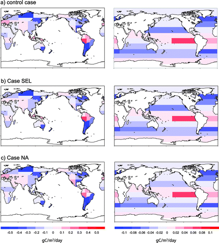
Fig. 9. Comparison of decadal mean (2002–2011) spatial distributions of posterior fluxes for the land biosphere (left panels) and ocean (right panels): (a) control case, (b) Case SEL, (c) Case NA. Positive fluxes indicate emission and negative fluxes indicate uptake.

Fig. 10. (a) Prior and posterior land fluxes and (b) uncertainty reduction (UR) in tropical Asia (Region 33) in the control case, Case CT, and Case NF. Positive fluxes indicate emission and negative fluxes indicate uptake.
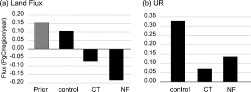
Fig. 10. (a) Prior and posterior land fluxes and (b) uncertainty reduction (UR) in tropical Asia (Region 33) in the control case, Case CT, and Case NF. Positive fluxes indicate emission and negative fluxes indicate uptake.

Fig. 11. Differences between estimated annual mean regional CO2 fluxes from the (a) land biosphere and (b) ocean derived with and without aircraft observations (control case – Case NA) during 2002–11. The numbered regions are shown in Fig. 3. Positive fluxes indicate emission and negative fluxes indicate uptake.
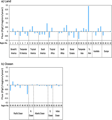
Fig. 11. Differences between estimated annual mean regional CO2 fluxes from the (a) land biosphere and (b) ocean derived with and without aircraft observations (control case – Case NA) during 2002–11. The numbered regions are shown in Fig. 3. Positive fluxes indicate emission and negative fluxes indicate uptake.

Fig. 12. Annually averaged atmospheric CO2 distributions at (a) 990 hPa, (b) 500 hPa, (c) 250 hPa, calculated from monthly pulsed emission from tropical Asia (Region 33) in 2008.
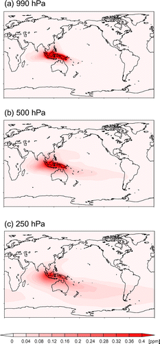
Fig. 12. Annually averaged atmospheric CO2 distributions at (a) 990 hPa, (b) 500 hPa, (c) 250 hPa, calculated from monthly pulsed emission from tropical Asia (Region 33) in 2008.

Fig. 13. Monthly mean land biosphere posterior fluxes (control case – red; Case NA – green) and prior fluxes (VISIT – gray), averaged over 2002–11. Positive fluxes indicate emission and negative fluxes indicate uptake.
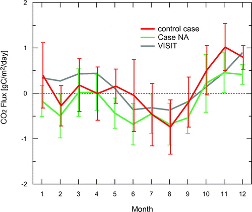
Fig. 13. Monthly mean land biosphere posterior fluxes (control case – red; Case NA – green) and prior fluxes (VISIT – gray), averaged over 2002–11. Positive fluxes indicate emission and negative fluxes indicate uptake.
Supplemental material

Supplementary Figure 2

Download PDF (321.7 KB)

Supplementary Figure 1

Download PDF (2.9 MB)