Variability in the correlation between satellite-derived liquid cloud droplet effective radius and aerosol index over the northern Pacific Ocean

Figures & data

Fig. 1. (a–d) The MODIS-derived climatological daily mean AOD, AI, precipitable water vapor (cm), and CER (μm) from 1 December 2002 to 31 December 2014. (e–h) the shaded images show the NCEP monthly long-term mean wind speeds (m s⁻¹) from 1981–2010 at the surface (e, g) and 500 hPa (f, h). Contour lines in (e, g) indicate sea level pressure (hPa) and contour lines in (f, h) indicate geopotential height (m). Rectangles A–E in (a–d) show the maps of the studied sea regions in the northern Pacific, A: the Bohai–Yellow Sea (32–41°N, 117°–127°E), B: the Sea of Japan (34–50°N, 127°–143°E), C: the western subarctic North Pacific (45–65°N, 145°E–180°E), D: the eastern subarctic North Pacific (45–65°N, 180°W–135°W), and E: the North Pacific subtropical gyre (15–35°N, 150°E–135°W).

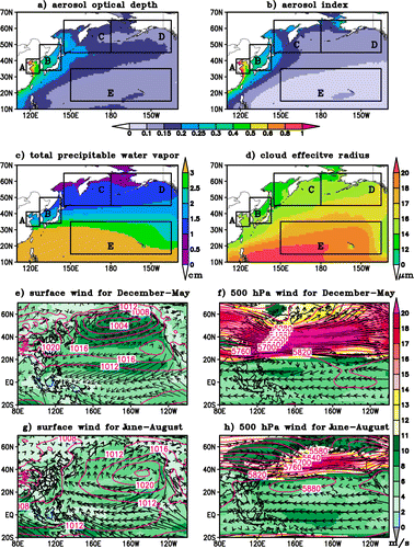
Fig. 2. Scatter plots of CER against AI in log scale over the five sea regions. (a–e) seasonal, (f) annual, (g) annual for CER at 3.7 μm. In (f) and (g), the letters a–e represent the five sea regions, respectively. The colours of points correspond to the colours of the letters. Data are from the MODIS Aqua Level 3 Collection 6 daily product MYD08_D3. The points represent CER sorted by AI, and both AI and CER are averaged over every 300 data points.

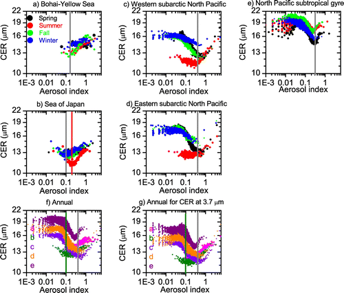
Table 1. Seasonal and annual correlation coefficients (R) and slopes (ACI_CER) of linear regression curves between aerosol index (AI) and cloud effective radius (CER) in log scale from 1 December 2002 to 31 December 2014.

Sea regions	AI range	Spring		Summer		Autumn		Winter		Annual
		R	ACICER	R	ACICER	R	ACICER	R	ACICER	R	ACICER
Bohai–Yellow Sea	≤0.1	1 data (–0.08)	1 data (–0.04)	2 data (–0.32) ^a	2 data (–0.07) ^a	−0.85^a	−0.05^a	1 data (–0.11)	1 data (–0.08)	2 data (–0.26)	2 data (–0.01)
	>0.1	0.19	0.01	0.95 ^b	0.07^b	0.83^b	0.09^b	0.56	0.02	0.87	0.05
	All	0.27	0.01	0.93	0.06	0.85	0.09	0.61	0.02	0.88	0.07
Sea of Japan	≤0.1	−0.21^e	−0.01^e	−0.81^c	−0.11^c	−0.67	−0.05	−0.73	−0.08	−0.71	−0.06
	>0.1	0.79^f	0.05^f	0.93^d	0.12^d	0.87	0.06	0.86	0.05	0.79	0.04
	All	0.58	0.02	0.41	0.04	0.59	0.03	0.62	0.03	0.71	0.04
Western subarctic North Pacific	≤0.4	−0.75	−0.15	−0.62	−0.03	−0.85	−0.07	−0.71	−0.02	−0.86	−0.08
	>0.4	0.76	0.09	0.97	0.13	0.66	0.05	0.89	0.04	0.82	0.09
	All	−0.81	−0.10	0.32	0.02	−0.86	−0.07	−0.70	−0.02	−0.86	−0.06
Eastern subarctic North Pacific	≤0.4	−0.95	−0.17	−0.13	−0.01	−0.75	−0.05	−0.42^e	−0.01^e	−0.80	−0.08
	>0.4	0.83	0.12	0.94	0.10	0.98	0.14	0.96^f	0.10^f	0.90	0.11
	All	−0.89	−0.14	0.30	0.01	−0.73	−0.05	−0.40	−0.01	−0.84	−0.06
North Pacific subtropical gyre	≤0.3	−0.73	−0.08	−0.45	−0.03	−0.80	−0.05	−0.83	−0.06	−0.73	−0.06
	>0.3	0.82	0.12	0.71	0.05	0.93	0.11	0.45	0.02	0.86	0.14
	All	−0.75	−0.08	−0.54	−0.03	−0.80	−0.05	−0.84	−0.06	−0.86	−0.07

Source: Bold numbers indicate significance at the 0.05 level. Values in parenthesis indicate that AI and CER were averaged over 50 data points or with no average, while the rest were averaged over 300 data points.

^a correlation is for AI ≤ 0.15.

^b correlation is for AI > 0.15.

^c correlation is for AI ≤ 0.2.

^d correlation is for AI > 0.2.

^e correlation is for AI ≤ 0.3.

^f correlation is for AI > 0.3.

Fig. 3. Correlation coefficients between AI and CER from 1 December 2002 to 31 December 2014 over the northern Pacific for different AI ranges. Rectangles A–E are the same as in Fig. 1.

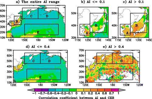
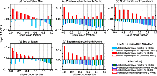
Fig. 4. Seasonal variation in the correlation coefficient (R) between AI and CER in log scale over the five sea regions. For each year, the sequence of the bars runs from spring (March, April, and May) to winter (December, January and February of the following year). The solid bars are statistically significant (p < 0.05) while the empty bars are not statistically significant (p > 0.05). The method is the same as in Fig. 2, but each point was averaged over every 50 data points. Each pair in one season in (c) and (d) represents R over the low (≤0.2, 0.3 or 0.4) and high (>0.2, 0.3 or 0.4) AI range, respectively.

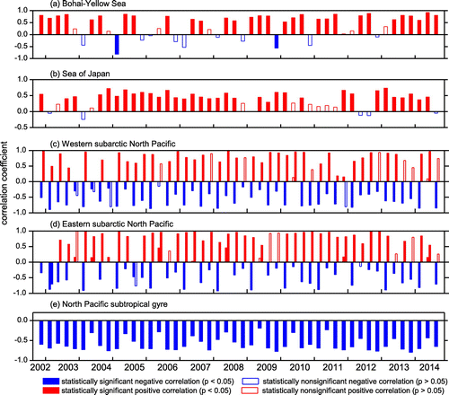
Fig. 5. Slopes of linear regression curves between AI and CER plots (ACI_CER) for 10 hPa cloud top pressure (CTP) intervals and 1 K cloud top temperature (CTT) intervals. Each ACI_CER in the figure is significant at the 0.05 level.

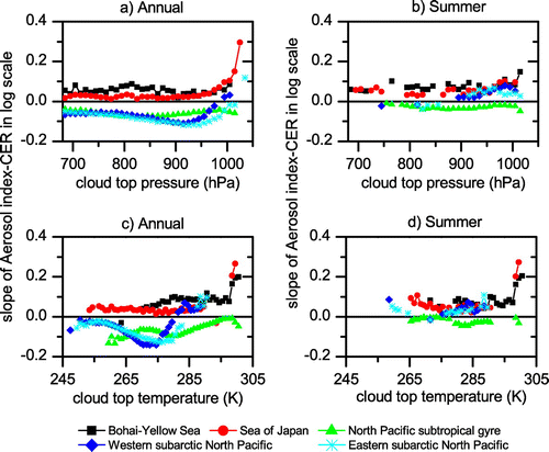
Table 2. Correlation coefficients (R) between monthly relative humidity (RH) or precipitable water vapour (PWV) and the regression slope (ACI_CER) and correlation coefficient (R[AI–CER]) of AI–CER in log scale, and p-values of the Granger causality test between them. The p-value of the Granger causality test is the significance level using the F distribution.

Sea regions	Bohai–Yellow Sea	Sea of Japan	Western subarctic North Pacific	Eastern subarctic North Pacific	North Pacific subtropical gyre
R between ACICER and PWV	0.37	0.02	0.28	0.28	0.60
R between R(AI–CER) and PWV	0.44	0.05	0.46	0.34	0.60
p-value for the test whether PWV Granger cause ACICER	1.05E-6	1.23E-06	3.58E-07	4.78E-05	9.44E-11
p-value for the test whether PWV Granger cause R[AI–CER]	4.81E-07	1.51E-05	2.93E-06	0.0002	7.63E-09
R between ACICER and RH	0.31	0.11	0.47	0.30	0.28
R between R[AI–CER] and RH	0.36	0.15	0.65	0.38	0.32
p-value for the test whether RH Granger cause ACICER	0.0001	3.05E-05	1.54E-05	0.40	5.00E-14
p-value for the test whether RH Granger cause R[AI–CER]	5.96E-05	0.0001	0.0002	0.37	5.86E-12

Source: All tests in this table are significant at the 0.05 level, except values in grey.

Fig. 6. (a -h) Dependence of the slopes of linear regression curves between AI and CER (ACI_CER) on precipitable water vapor (PWV, cm) for 10 or 30 g m⁻² LWP intervals; (i) Dependence of ACI_CER on PWV for total LWP; (j) Dependence of ACI_CER on lower tropospheric stability. Each ACI_CER in the figure is significant at the 0.05 level.

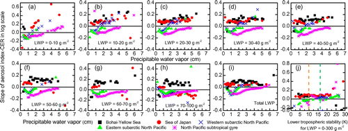
Table 3. Correlation coefficients of linear regression between the slope of the AI–CER curve in log scale (ACI_CER) and precipitable water vapour (PWV) for different liquid water path (LWP) intervals.

LWP intervals	Bohai–Yellow sea	Sea of Japan	Western subarctic North Pacific	Eastern subarctic North Pacific	North Pacific subtropical gyre
0–10	0.95	0.88	0.98	0.69	0.98
10–20	0.93	−0.02	0.95	0.76	0.35
20–30	0.87	0.65	0.90	0.86	0.97
30–40	0.50 (0.90)	0.11	0.92	0.86	0.95
40–50	0.61 (0.94)	0.48	0.54	0.85	0.97
50–60	0.41 (0.98)	−0.88	0.84	0.90	0.98
60–70	0.61 (0.88)	0.11	0.51	0.21	0.94
70–100	0.44 (0.98)	−0.91	−0.59	0.46	0.97
0–100/Mean	0.70 (0.92)	0.52	0.81	0.90	0.88
All LWP	0.32 (0.98)	0.004	0.62	0.78	0.95

Source: Values in the parenthesis show correlation coefficients for PWV < 1.5 cm. Bold numbers are significant at the 0.05 level.

Fig. 7. Scatter plots of precipitable water vapour (cm) and relative humidity (%) against AI and CER over the two marginal seas. Each point was obtained in the same manner as in Fig. 2.

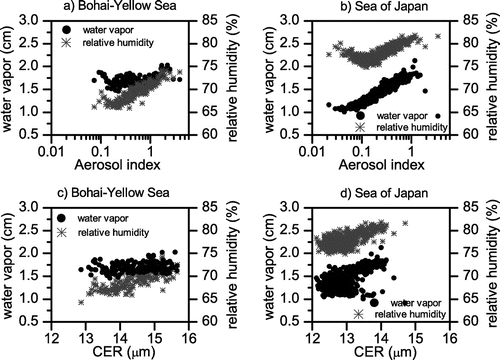
Fig. 8. The slope of linear regression curves between AI and CER (ACI_CER) in 10 10% liquid cloud fraction (LCF) intervals over the 5 sea regions. Each pair in one 10% LCF intervals represents the ACI_CER over the low, high and entire AI range, respectively. The solid bars are statistically significant (p < 0.05) while the empty bars are not statistically significant (p > 0.05).