Sensitivity assessment of PM_2.5 simulation to the below-cloud washout schemes in an atmospheric chemical transport model

Figures & data

Table 1. Raindrop size distributions extracted from the literature.

	References	Formula
A	Marshall and Palmer (1948)^a^,1	N0 = 8$\times$10^6, $\alpha$ = 0, $\gamma$ = 1,$\beta$ = 4100P^−0.21
B	Ulbrich (1983)^a^,1	N0 = 5.1$\times$10^6P^−0.03, $\alpha$ = 0, $\gamma$ = 1, $\beta$ = 3800P^−0.2
C	Cerro et al. (1997)^a^,1	N0 = 2.32$\times$10^6P^0.22, $\alpha$ = 0, $\gamma$ = 1, $\beta$ = 4000P^−0.1065
D	De Wolf (2001)^a^,1	N0 = 1.22$\times$10^1^6P^−0.384, $\alpha$ = 2.93, $\gamma$ = 1, $\beta$ = 5380P^−0.186
E	Chapon et al. (2008)^a^,1	N0 = 7.5$\times$10^1^8P^0.001, $\alpha$ = 3.47, $\gamma$ = 1, $\beta$ = 7640P^−0.214
F	Chen et al. (2013)^a^,2	N0 = 2.1$\times$10^4, $\alpha$ = 3.51, $\gamma$ = 1, $\beta$ = 4.52
G	Aoki et al. (2016)^a^,2	N0 = 8.3$\times$10^3, $\alpha$ = 2.3, $\gamma$ = 1, $\beta$ = 3.2
H	Das et al. (2017)^a^,2	N0 = 3.16$\times$10^6, $\alpha$ = 7.9, $\gamma$ = 1, $\beta$ = 9.9
I	Chen et al. (2017)^a^,2	N0 = 610, $\alpha$ = −0.158, $\gamma$ = 1, $\beta$ = 2.26
J	Feingold and Levin (1986)^b	Ntot = 1.72$\times$10^2P^0.22, Dmean = 7.2$\times$10^−4P^−0.23, ${\sigma }_D$ = 1.43–3$\times$10^−4P
K	Timothy et al. (2002)^b	Ntot = 2.03$\times$10^2P^0.241, Dmean = e^−0.313 + 0.227ln^P$\times$10^−3, ${\sigma }_D$ = $e^{\sqrt{0.108-0.0086\ln P}}$
L	Harikumar et al. (2010)^b	Ntot = 2.68$\times$10^2P^0.308, Dmean = 5.96$\times$10^−4P^−0.216, ${\sigma }_D$ = 1.55–0.0217lnP

^a Gamma distribution: $N(D)=N_0{D}^{\alpha }\exp (-\beta D^{\gamma })$. When $\alpha$ = 0, $\gamma$ = 1, the equation then becomes the exponential distribution.

¹ N₀ unit is in m⁻³ m^−1-α, β unit is in m^−γ.

² N₀ unit is in m⁻³ mm^−1-α, β unit is in mm^−γ.

^b Log-normal distribution: $N(D)=\frac{N_{tot}}{\sqrt{2\pi }D\ln ({\sigma }_D)}\exp \left[-\frac{{(\ln (D)-\ln (D_{mean}))}^2}{2{(\ln ({\sigma }_D))}^2}\right]$. N_tot is in m⁻³, D_mean is in m.

Fig. 1. (a–c): WRF (dash line) and CAMx (solid line) domain setting. Blue dots and red numbers represent the locations of the ground-based PM2.5 observation station and precipitation observation station, respectively. ‘SZ’ represents Shenzhen, ‘HK’ represents Hong Kong, ‘HZ’ represents Huizhou, ‘DG’ represents Dongguan, ‘ZS’ represents Zhongshan, ‘ZH’ represents Zhuhai, ‘JM’ represents Jiangmen, ‘ZQ’ represents Zhaoqing, ‘GZ’ represents Guangzhou, and ‘FS’ represents Foshan.

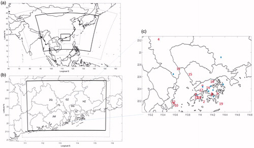
Fig. 2. (A–B): Simulated geographic distribution of accumulated precipitation mapping (by WRF) in the PRD region during September 3–13, 2010 (A). The numbers on the x-axis in subfigure B represent different precipitation observation stations. The geological locations of these stations can be found in Fig. 1c, marked by red numbers.

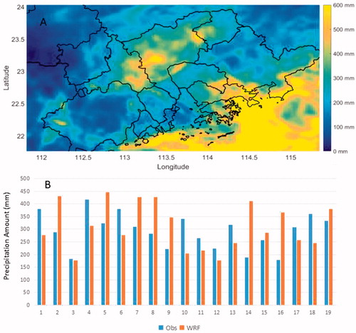
Table 2. Model statistical metrics using different BCW schemes.

Case	Scheme	Mean	MB	ME	NMB	NME
A	CAMx v6.00	26.5	4.1	17.0	0.20	0.77
B	CAMx v6.40	18.9	−3.5	14.9	−0.15	0.67
C	Loosmore et al. (2004)	25.3	2.9	16.9	0.15	0.76
D	AURAMS	25.2	2.8	16.4	0.14	0.74
E	EMEP	24.1	1.7	16.0	0.09	0.72
F	CMAQ	11.9	−10.5	14.9	−0.47	0.67
G	CALPUFF	16.0	−6.4	14.9	−0.28	0.67
H	ADMS	16.6	−5.8	14.6	−0.26	0.65
I	Sparmacher et al. (1993)	26.0	3.6	16.8	0.18	0.76
J	Laakso et al. (2003)	23.5	1.1	15.6	0.06	0.70
K	Wang et al. (2014c)	20.2	−2.2	14.3	−0.09	0.64
L	Baklanov and Sorensen. (2001)	16.9	−5.5	14.7	−0.24	0.66
M	Kang et al. (2015)	26.5	4.1	17.0	0.20	0.77
N	Wang et al. (2014a)	26.3	3.9	16.9	0.19	0.75
	Observations	22.4

‘Mean’ represents the mean PM_2.5 concentration over the 10 observation stations in the study period; ‘MB’ represents the mean bias; ‘ME’ represents the mean error; ‘NMB’ represents the normalized mean bias; ‘NME’ represents the normalized mean error. The lowest values for MB, ME, NMB and NME are bolded.

Fig. 3. Time series of PM_2.5 simulation using different BCW schemes at Tung Chung (a), Tai Po (b), Tsuen Wan (c), and Wanqingsha (d) stations.

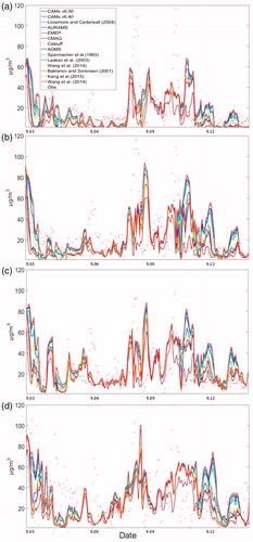
Fig. 4. Spatial difference (compared to CAMx v6.40) of PM_2.5 simulation by using different BCW schemes (Unit: %). Letter labels on the panels refer to the simulations described in Table 2.

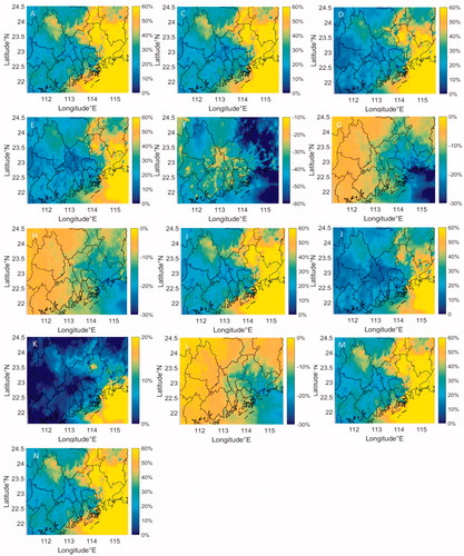
Table 3. PM_2.5 average simulated concentration (μg m⁻³) by different BCW schemes for each city during the study period.

City*	A	B	C	D	E	F	G	H	I	J	K	L	M	N
HZ	20.1	12.7	19.4	18.8	17.9	6.9	10.3	10.7	19.7	18.3	13.8	11.0	20.1	20.1
GZ	40.2	30.2	38.7	38.6	36.5	20.2	26.1	26.8	39.4	37.4	31.3	27.2	40.1	40.1
FS	40.6	33.5	39.8	39.3	38.3	24.6	30.1	30.6	40.1	38.7	34.1	31.0	40.6	40.6
DG	44.3	35.1	42.9	42.8	41.1	24.5	29.5	30.6	43.6	41.6	36.0	30.9	44.2	44.2
JM	21.4	17.1	20.9	20.2	20.2	11.5	15.7	15.8	21.1	20.4	17.3	16.1	21.3	21.4
SZ	35.8	27.1	34.4	34.5	32.8	18.4	22.7	23.7	35.3	33.5	28.6	23.9	35.8	35.8
ZS	30.9	24.3	29.9	29.6	28.8	17.1	21.5	22.0	30.4	29.1	25.0	22.3	30.8	30.8
ZQ	27.2	21.4	26.8	25.9	25.8	14.5	19.7	19.9	26.9	26.0	21.9	20.3	27.2	27.2
HK	22.1	15.0	20.9	20.9	19.8	8.8	12.5	13.0	21.7	20.3	16.3	13.3	22.1	22.1
ZH	23.2	17.5	22.3	22.0	21.4	12.1	15.8	16.1	22.8	21.9	18.3	16.3	23.1	23.2

* The cities are identified in Fig. 1.

Table 2 describes the simulations A-N and Fig. 1 defines the city acronyms and shows their locations.

Fig. 5. Time series of PM_2.5 simulation using different raindrop size distribution parameterizations at Tung Chung (a), Tai Po (b), Tsuen Wan (c) and Wanqingsha (d) stations.

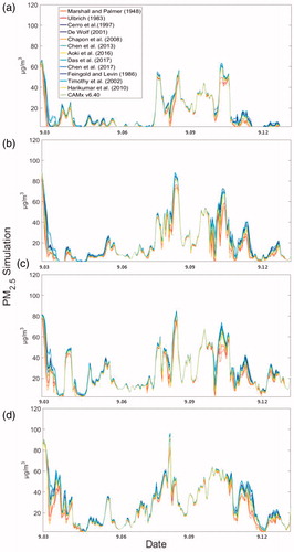
Fig. 6. Spatial difference (compared to CAMx v6.40) of PM_2.5 simulation by using different raindrop size distribution parameterizations (Unit: %). Letter labels on the panels refer to the simulations described in Table 1.

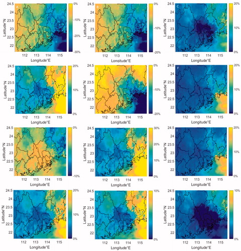
Table 4. Source contribution (in %) to the sum of three PM_2.5 components (, and ).

	CAMx v6.40			CAMx v6.00			EMEP
City	Local	Regional	S-regional	Local	Regional	S-regional	Local	Regional	S-regional
HZ	23.0	19.6	57.4	17.3	16.4	66.4	18.4	16.7	64.9
GZ	30.2	17.8	52.0	26.7	16.0	57.4	27.4	16.3	56.3
FS	29.3	19.1	51.5	26.3	17.1	56.6	26.9	17.5	55.6
DG	23.9	33.0	43.1	18.6	28.8	52.6	19.8	29.8	50.4
JM	21.2	8.6	70.2	19.5	7.7	72.8	19.8	7.8	72.3
SZ	34.5	26.3	39.2	26.9	22.8	50.3	28.7	23.5	47.8
ZS	20.1	25.8	54.1	18.2	22.0	59.8	18.7	22.8	58.6
ZQ	18.9	15.4	65.7	17.6	13.7	68.7	17.8	13.8	68.3
HK	18.4	33.0	48.6	15.1	24.4	60.5	16.0	26.2	57.8
ZH	16.3	21.3	62.4	14.3	17.2	68.5	14.9	18.2	67.0

Figure 1 defines the city acronyms and shows their locations.

Table 5. The BCW coefficients calculated by field observation data at the HKUST super-site.*

Time (DD_HHMM)	(s^−1)	(s^−1)	(s^−1)	Precip (mm)	Duration (min)
6.06_6:00-7:59	1.9 × 10^−4	3.4 × 10^−4	8.7 × 10^−5	16.8	21
6.08_1:00-5:59	4.5 × 10^−4	3.2 × 10^−4	2.7 × 10^−4	35.0	72
6.10_18:00-18:59	3.6 × 10^−4	3.2 × 10^−4	2.5 × 10^−4	10.9	26
6.10_21:00-21:59	5.9 × 10^−4	5.6 × 10^−4	4.0 × 10^−4	5.6	15
6.11_11:00-12:59	−5.1 × 10^−5	2.4 × 10^−4	1.2 × 10^−4	12.4	43
6.12_7:00-8:59	−1.1 × 10^−4	1.9 × 10^−4	5.1 × 10^−5	10.7	32
6.12_10:00-10:59	2.4 × 10^−4	−1.7 × 10^−4	3.9 × 10^−4	4.3	15
6.17_4:00-4:59	2.9 × 10^−4	7.7 × 10^−4	1.4 × 10^−4	5.8	13
6.17_7:00-7:59	2.0 × 10^−4	2.8 × 10^−4	1.7 × 10^−4	8.4	17
7.09_22:00-22:59	−3.0 × 10^−5	4.7 × 10^−4	−9.5 × 10^−5	10.4	16
7.11_3:00-3:59	2.7 × 10^−4	3.9 × 10^−4	1.9 × 10^−4	4.3	12
7.11_6:00-6:59	6.9 × 10^−5	2.2 × 10^−4	9.0 × 10^−5	11.9	21
7.13_7:00-7:59	2.4 × 10^−5	8.3 × 10^−5	2.2 × 10^−5	15.5	41
7.14_12:00-12:59	1.6 × 10^−4	2.7 × 10^−4	2.8 × 10^−5	4.1	13
8.10_7:00-7:59	2.7 × 10^−4	5.0 × 10^−4	3.3 × 10^−4	39.6	60
8.11_9:00-11:59	7.1 × 10^−5	1.5 × 10^−4	4.7 × 10^−5	14.2	45
8.28_1:00-2:59	6.4 × 10^−4	3.4 × 10^−4	8.8 × 10^−4	14.5	35
Median	2.0 × 10^−4	3.2 × 10^−4	1.4 × 10^−4	–	–

* The HKUST super-site is in Clear Water Bay, Kowloon, Hong Kong.

Marshall, J. S. and Palmer, W. M. K. 1948. The distribution of raindrops with size. J. Meteor. 5, 165–166. DOI:10.1175/1520-0469(1948)005<0165:TDORWS>2.0.CO;2.

 Google Scholar

Ulbrich, C. W. 1983. Natural variations in the analytical form of the raindrop size distribution. J. Climate Appl. Meteor. 22, 1764–1775. DOI:10.1175/1520-0450(1983)022 < 1764:NVITAF >2.0.CO;2.

 Google Scholar

Cerro, C., Codina, B., Bech, J. and Lorente, J. 1997. Modeling raindrop size distribution and Z (R) relations in the Western Mediterranean area. J. Appl. Meteor. 36, 1470–1479. DOI:10.1175/1520-0450(1997)036<1470:MRSDAZ>2.0.CO;2.

 Google Scholar

de Wolf, D. A. 2001. On the Laws-Parsons distribution of raindrop sizes. Radio Sci. 36, 639–642.

 Web of Science ®Google Scholar

Chapon, B., Delrieu, G., Gosset, M. and Boudevillain, B. 2008. Variability of rain drop size distribution and its effect on the Z–R relationship: A case study for intense Mediterranean rainfall. Atmos. Res. 87, 52–65. DOI:10.1016/j.atmosres.2007.07.003

 Web of Science ®Google Scholar

Chen, B., Yang, J. and Pu, J. 2013. Statistical characteristics of raindrop size distribution in the Meiyu season observed in Eastern China. J. Meteorol. Soc. Japan. 91, 215–227. 85. DOI:10.2151/jmsj.2013-208.

 Web of Science ®Google Scholar

Aoki, M., Iwai, H., Nakagawa, K., Ishii, S. and Mizutani, K. 2016. Measurements of rainfall velocity and raindrop size distribution using coherent Doppler lidar. J. Atmos. Ocean Tech. 33, 1949–1966. DOI: 10.1175/JTECH-D-15-0111.1

 Web of Science ®Google Scholar

Das, S. K., Konwar, M., Chakravarty, K. and Deshpande, S. M. 2017. Raindrop size distribution of different cloud types over the Western Ghats using simultaneous measurements from Micro-Rain Radar and disdrometer. Atmos. Res. 186, 72–82. DOI:10.1016/j.atmosres.2016.11.003

 Web of Science ®Google Scholar

Chen, B., Hu, Z., Liu, L. and Zhang, G. 2017. Raindrop Size Distribution Measurements at 4,500 m on the Tibetan Plateau During TIPEX-III. J. Geophys. Res, 122. DOI: 10.1002/2017JD027233

 Web of Science ®Google Scholar

Feingold, G. and Levin, Z. 1986. The lognormal fit to raindrop spectra from frontal convective clouds in Israel. J. Climate Appl. Meteor. 25, 1346–1363. DOI:10.1175/1520-0450(1986)025<1346:TLFTRS>2.0.CO;2.

 Google Scholar

Timothy, K. I., Ong, J. T. and Choo, E. B. 2002. Raindrop size distribution using method of moments for terrestrial and satellite communication applications in Singapore. IEEE Trans. Antennas Propag. 50, 1420–1424. DOI: 10.1109/TAP.2002.802091

 Web of Science ®Google Scholar

Harikumar, R., Sampath, S. and Kumar, V. S. 2010. Variation of rain drop size distribution with rain rate at a few coastal and high altitude stations in southern peninsular India. Adv. Space Res. 45, 576–586. DOI: 10.1016/j.asr.2009.09.018

 Web of Science ®Google Scholar

Loosmore, G. A. and Cederwall, R. T. 2004. Precipitation scavenging of atmospheric aerosols for emergency response applications: testing an updated model with new real-time data. Atmos. Environ. 38, 993–1003. DOI:10.1016/j.atmosenv.2003.10.055.

 Web of Science ®Google Scholar

Sparmacher, H., Fülber, K. and Bonka, H. 1993. Below-cloud scavenging of aerosol particles: Particle-bound radionuclides—Experimental. Atmos. Environ.. Part A. Gen. Top. 27, 605–618. DOI:10.1016/0960-1686(93)90218-N.

 Web of Science ®Google Scholar

Laakso, L., Grönholm, T., Rannik, Ü., Kosmale, M., Fiedler, V. and co-authors. 2003. Ultrafine particle scavenging coefficients calculated from 6 years field measurements. Atmos. Environ. 37, 3605–3613. DOI:10.1016/S1352-2310(03)00326-1.

 Web of Science ®Google Scholar

Wang, Y., Zhu, B., Kang, H., Gao, J., Jiang, Q. and co-authors. 2014c. Theoretical and observational study on below-cloud rain scavenging of aerosol particles. J. Univ. Chin. Acad. Sci.. 31, 306–313. In Chinese).

 Google Scholar

Baklanov, A. and Sørensen, J. H. 2001. Parameterisation of radionuclide deposition in atmospheric long-range transport modelling. Phys. Chem. Earth. Part B: Hydrology, Oceans and Atmosphere 26, 787–799. DOI:10.1016/S1464-1909(01)00087-9.

 Web of Science ®Google Scholar

Kang, Y., Hua, F., Zhong, K. and Zhu, H. 2015. A new analysis of fine aerosol capture by raindrops at terminal velocities. J. Aero. Sci. 89, 31–42. DOI:10.1016/j.jaerosci.2015.06.007.

 Web of Science ®Google Scholar

Wang, X., Zhang, L. and Moran, M. D. 2014a. Development of a new semi-empirical parameterization for below-cloud scavenging of size-resolved aerosol particles by both rain and snow. Geosci. Model Dev. 7, 799–819. DOI:10.5194/gmd-7-799-2014.

 Web of Science ®Google Scholar