
Figures & data
Fig. 1. (a) Map of central Sweden showing the sampling site, Mt Åreskutan (black square), the start point of the Västmanland forest fire (black triangle), Digernäset station (pale blue dot), Medstugan station (blue dot), Vallbo station (red dot) and Stockholm (blue square) for reference. (b) Custom-built active strand cloudwater collector (Collett et al., Citation1990) used during the CAEsAR 2014 campaign.
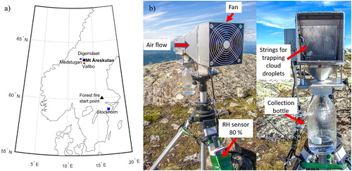
Table 1. Sample type, ID, sampling period, and amount of water collected of rain and fog samples taken during the CAEsAR 2014 campaign.
Table 2. Mean molar concentrations, standard deviation (1σ), 25th, 50th, and 75th percentiles of selected ions, δ(15N), δ(18O), δ(17O), and Δ(17O) in rain and fog samples.
Fig. 2. Pie-plot of ion fractions (mol-%) measured in (a) rain and (b) fog samples during the CAEsAR campaign. Nss- and ss-fractions were calculated as explained in Section 2.2.
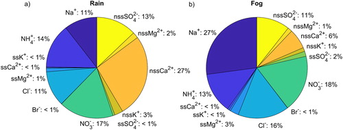
Fig. 3. Sea-salt ratios referred to Na+ in bulk seawater (blue diamonds), in rain (black circles) samples, and in fog (red stars) samples collected during the CAEsAR campaign. Fog/rain ratios were calculated using mean ion concentrations. Error bars represent 1σ.
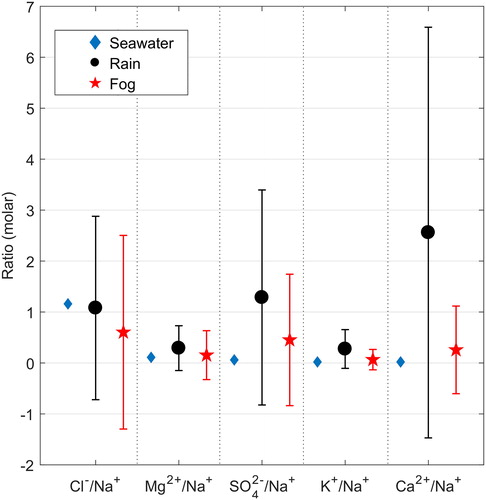
Table 3. PCA loadings of the first three principal components calculated using concentrations of major ions (separated into ss- and nss-fractions) measured in rain and fog samples collected during the CAEsAR 2014 campaign.
Fig. 4. Stacked bar plot of NH4+, NO3−, and Na+ concentrations in each (a) rain and (b) fog sample collected during the CAEsAR campaign. Horizontal arrows indicate that samples R6 and R7 overlap with sample F8; while samples R9 and R10 together overlap with sample F10 and F11. For sample collection periods see .
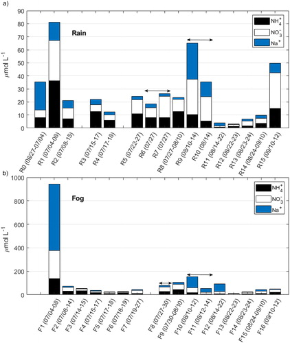
Fig. 5. Stacked bar plot of Br−, nssMg2+, nssSO42−, and K+ concentrations in each (a) rain and (b) fog sample collected during the CAEsAR campaign. Note that Br− concentrations have been scaled to improve visualization. Horizontal arrows indicate that samples R6 and R7 overlap with sample F8; while samples R9 and R10 together overlap with sample F10 and F11. For sample collection periods please refer to .
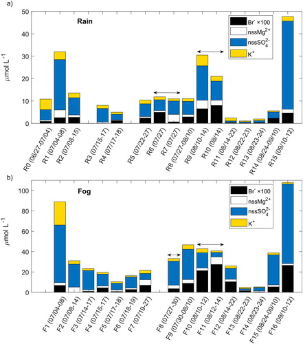
Table 4. Rain and fog sample classification considering concentrations thresholds; more than double the mean (high), less than half the mean (low), and within twice the mean and half the mean (medium).
Fig. 6. 7-day back-trajectories arriving to Åreskutan for samples (a) R1, (b) R9, (c) R8, (d) R15, (e) R12, and (f) R13. Start altitude is an elevation of 500 m above ground level (a.g.l.). Each colour represents a back-trajectory restarted each 48 h: initial back-trajectory (red line and triangles), restarted after 48 h (blue line and squares), and restarted after 96 h (green line and circles).
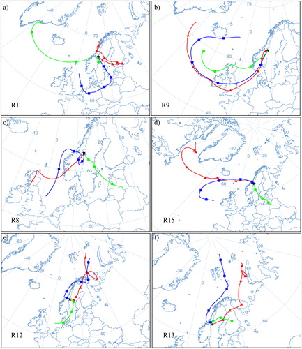
Fig. 7. Stacked bar plot of (a) NH4+, and NO3−, and (b) Br−, nssMg2+, and nssSO42− daily rain deposition obtained as explained in Section 2.3. Note that Br− concentrations have been scaled to improve visualization.
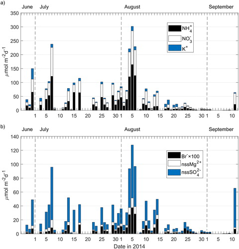
Fig. 8. Bar plot of (a) δ(15N), and (b) δ(18O) and Δ(17O) in NO3−, from rain and fog samples collected during the CAEsAR campaign. In the bottom graph, Δ(17O) values for rain and fog samples are shown with red and blue lines, respectively. (*) The sampling date is (as detailed in ): R5 07/22–27, R7 07/27, F9 07/30–08/10, F10 08/10–12.
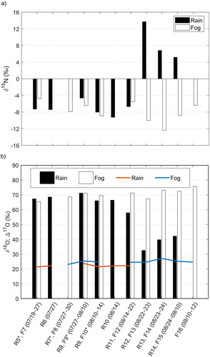
Table 5. Fog/rain ratios of mean ion concentrations of samples classified as high, medium, or low (explained in Section 3.2), and associated to three main ion sources: anthropogenic (i.e. high NO3− concentrations), inland (i.e. medium NO3− concentrations), and marine Arctic (i.e low NO3− concentrations), also described in Section 3.2.
Table 6. Mean and standard deviation (1σ) for rain and fog deposition of selected ions considering modelled deposition velocities reported by Matsumoto et al. (Citation2011).
Table S1. Mean daily precipitation estimated as the mean of daily precipitation at the three SMHI stations near Åre: Medstugan, Digernäset and Vallbo, and mean, median, standard deviation (1σ), maximum, and minimum precipitation values for the three stations (considering the study period, i.e., 77-days).
Table S2. Days in which fog was present at the sampling site and mean liquid water content γ(H2O), for each sample interval.
Supplemental Material
Download PDF (823.6 KB)Data availability
Precipitation data for Medstugan, Digernäset, and Vallbo stations was provided by the Swedish Meteorological and Hydrological Institute (SMHI, http://opendata-download-metobs.smhi.se). Back-trajectories obtained using the HYSPLIT model can be retrieved using the online platform of the model from the NOAA Air Resources Laboratory (https://ready.arl.noaa.gov/HYSPLIT_traj.php). The data collected in this study are available upon request to the corresponding author.