Figures & data
Fig. 1. Location of sites in France.
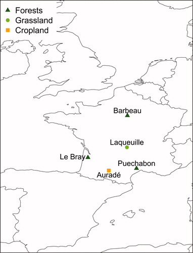
Table 1. Experimental sites characteristics.
Table 2. Setup at each site. Tair stands for air temperature at measurement height (in °C), RH for relative humidity (in %), Sd for incoming shortwave radiation (in W m−2), u for wind speed (in m s−1), P for precipitation (in mm), θ for soil water content (in mm).
Fig. 2. RF analysis results: importance of environmental variables explaining the variability of carbon fluxes (A. NEE, B. GPP and C. Reco) at a half-hourly time-step at five ecosystem stations. Standard deviation on the mean of %imp of each environmental variable, computed from a bootstrap analysis (n = 100), were voluntarily omitted in the graph as they presented values lower than 0.1% in each case (See Supplementary material S3.1).
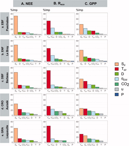
Table 3. Input parameters optimization and results of the RF approach in terms of percentage of variance explained from the half-hourly (five sites), daily, monthly and seasonal (two sites selected) time scales. « ndata » corresponds to the number of data in the time-step considered; « mtry » stands for the number of explanatory variables to randomly sample as candidates at each split and « ntrees » for the number of trees in the RF analysis.
See Supplementary material (§ S3.1) for further information.
Fig. 3. RF analysis results: importance of environmental variables explaining the carbon flux variabilities for Puechabon (A) and Auradé (B) at different time scales. Standard deviation on the mean of %imp of each environmental variable, computed from a bootstrap analysis (n = 1000), were voluntarily omitted in the graph as they presented values lower than 1.5% for each case (§ S3.1).
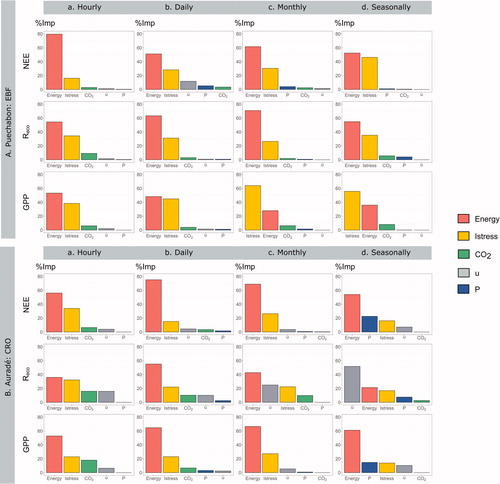
Fig. 4. 2006–2011 monthly time series of environmental variables (Sd, Tair, Cumulative P, u and D) for the three sites selected in the wavelet analyses.
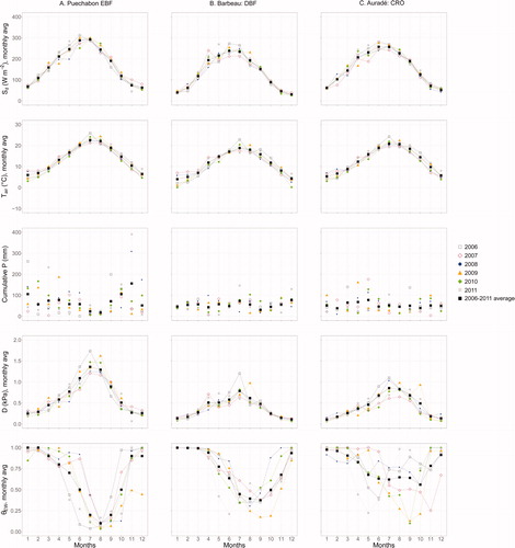
Fig. 5. 2006–2011 monthly time series of carbon fluxes (NEE, GPP, and Reco), for the three sites selected in the wavelet analyses.
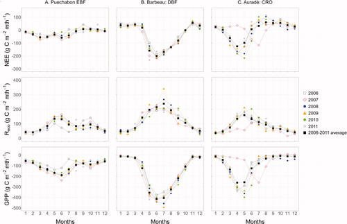
Fig. 6. Wavelet Power Spectra (WPS) of environmental variables (scalograms) and corresponding profile of the average wavelet power (curves) at three sites (Puechabon, Barbeau and Auradé).
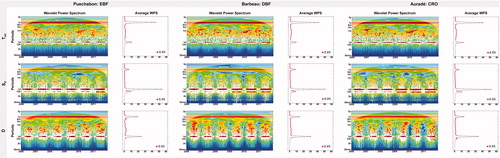
Fig. 7. Wavelet Power Spectra (WPS) of ecosystem carbon fluxes (scalograms) and corresponding profile of the average wavelet power (curves) at three sites (Puechabon, Barbeau and Auradé).
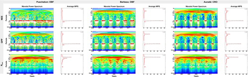
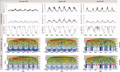
Fig. 8. Cross-wavelet coherence (CWC) analysis of GPP (B) and Reco (C) with D at three sites (Puechabon, Barbeau and Auradé) from 2006 to 2011. The monthly time series of variables (A) are presented together with the corresponding scalograms of CWC. The red colour indicates high coherence between the two-time series at a particular time and a particular period. A blue one indicates no coherence between the two time series. Arrows on the cross-wavelet coherence plots stand for the synchronization analyses and are plotted only within white contour lines indicating significance (with respect to the null hypothesis of white noise processes) at the 5% level. Arrows are pointing right for the in-phase two series relationship (e.g., positively correlated with no lags), left for the anti-phase relationship (e.g., negatively correlated with no lags), and straight up (down) when carbon flux (biometeorological variable) is leading the biometeorological variable (carbon flux) by π/2 radians. Finally, the grey zone represents the cone of influence in which the spectral information is likely to be less accurate (Torrence & Compo Citation1998).
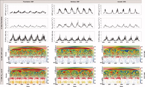
Fig. 9. Cross-wavelet coherence (CWC) analysis of GPP (B) and Reco (C) with θEW at three sites (Puechabon, Barbeau and Auradé) from 2006 to 2011. The monthly time series of variables (A) are presented together with the corresponding scalograms of CWC.