Figures & data
Table 1. Reproducibility tests of laboratory 14ΔCO2 measurements.
Fig. 1. Variation of atmospheric Δ14CO2 level (within 1σ) as a function of northward increasing latitude.
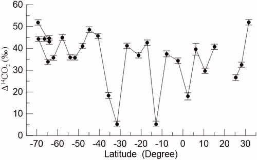
Table 2. In situ records, levels of atmospheric δ13CO2 and Δ14CO2, and statistics of vertical trajectories of the samples.
Fig. 2. Three-dimensional 96-h backward trajectories of the sampled air parcels: (a) samples #15–#29 covering the Western Australia coastline, southeast Asia ITCZ, and subtropical western Pacific, (b) samples #1–#14 covering the Southern Ocean and the coastal region of East Antarctica.
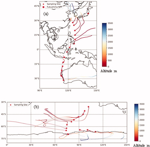
Fig. 3. (Upper) MBL Δ14CO2 level from 68.0°S to 64.0°S and (lower) the vertical cross section of in situ measured ocean temperature isotherms along 74.0°E. The red rectangle in the inset of the lower panel; represents the R/V Xuelong track positions, along which the vertical section of water temperature contours is plotted.
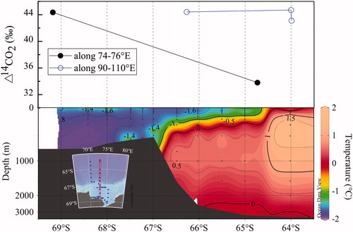
Fig. 4. (Upper) Spatial variation of MBL Δ14CO2 from ∼70.0°S to the equator along the Xuelong cruise track during the 27th CHINARE and (lower) the corresponding vertical cross section of ocean water salinity contours. The red lines in the inset of the lower panel represent the R/V Xuelong track, along which the vertical section of the salinity contours is plotted.
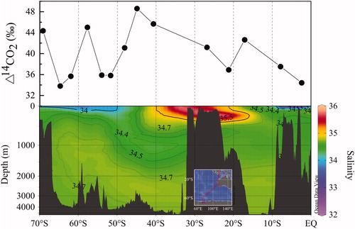
Fig. 5. Hourly averages of surface ozone at Zhongshan corresponding to date of atmospheric Δ14CO2 sampling: (a) sample #1 on 6 January 2011 and (b) sample #5 on 26 February 2011.
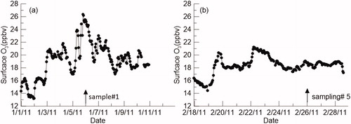
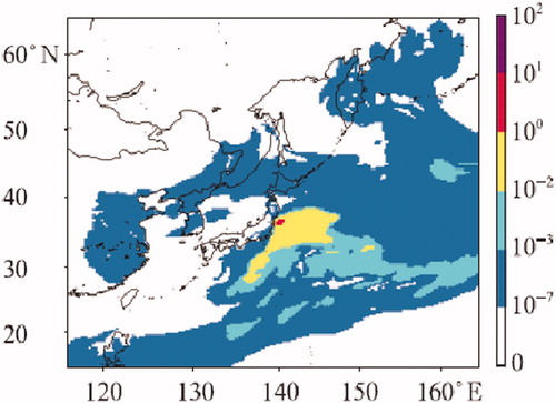
Fig. 6. Distribution of depositional radioactive particles (A25J) from the Fukushima NPP accident at 09:00 (UTC) on 29 March 2011 simulated by Model-3/CMAQ (Xiangwang et al., Citation2012).