Figures & data
Figure 1. Exploration for three cuproptosis-related MM subtypes. (A) Cumulative distribution function (CDF) curve, CDF delta area curve as well as the delta area curve of consensus clustering of samples from UCSC Xena exhibiting the relative alterations in the area under the CDF curve for each category number k compared with category number k-−1. (B) Sample clustering heatmap when consensus k = 3. (C) Survival analyzes for the three clusters (P < 0.0001). (D) Heatmap of cuproptosis-related genes expression in MM samples with different clinical data. (E) Correlation bubble diagram among cuproptosis genes. (F) The correlation network among cuproptosis genes.
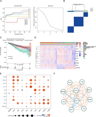
Figure 2. Identification and evaluation of candidate cuproptosis related genes and candidate genes. (A) Volcano plot of 346 DEGs between Cluster 3 and Cluster 1. (B) Volcano plot of 2931 DEGs between MM and normal samples in GSE47552. (C) Volcano plot of 2817 DEGs between MM and normal samples in GSE16558. For a–c, the screening criteria are set to P < 0.05, | log2foldchange | ≥ 0.5. (D) Venn diagrams for up-regulated and down-regulated intersecting genes by overlapping DEGs and candidate cuproptosis related genes. (E) Heatmap for candidate genes expression between MM and normal samples in GSE47552. (F) Heatmap for 33 candidate genes expression between MM and normal samples in GSE16558. (G)The Gene Ontology (GO) analysis for candidate genes, including the enriched biological processes, cellular composition terms. (H) The top 4 enriched Kyoto Encyclopedia of Genes and Genomes (KEGG) terms of candidate genes.
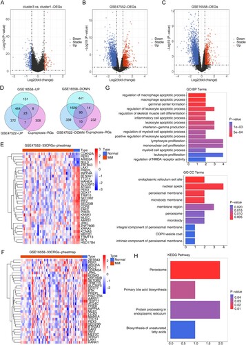
Table 1. Gene expression patterns of candidate genes.
Figure 3. Identification of prognostic genes (A) Forest map for univariate Cox analysis to screen six survival related cuproptosis genes. (B) Kaplan–Meier (K–M) survival curve of 784 MM samples with different expressed patterns of six survival related cuproptosis genes, including CDKN2A (P < 0.0001), BCL3 (P = 0.018), KCNA3 (P = 0.0019), TTC14 (P = 0.0053), XRRA1 (P = 0.00093), and SLC35F5 (P < 0.38). (C) Least absolute and selection operator (LASSO) regression analysis to screen prognostic genes. LASSO coefficient profiles (top) and cross-validation (bottom) to select the optimal tuning parameter.
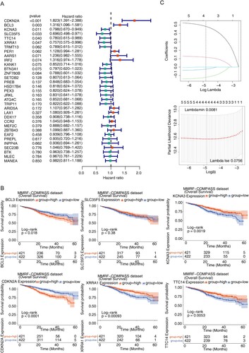
Table 2. Four model genes screened using LASSO COX regression analysis.
Figure 4. Construction and assessment of the prognostic risk model. (A) Risk score curve, survival status and gene expression of four prognostic genes between high- and low-risk groups in training set. (B) K–M survival curve of high- and low-risk groups in training set (P < 0.0001). (C) Receiver operating characteristic (ROC) curves of training set. (D) Risk score curve, survival status and gene expression of four prognostic genes between high- and low-risk groups in validation set (GSE4581). (E) K–M survival curve of high- and low-risk groups in validation set. (F) ROC curves of validation set (P < 0.005).
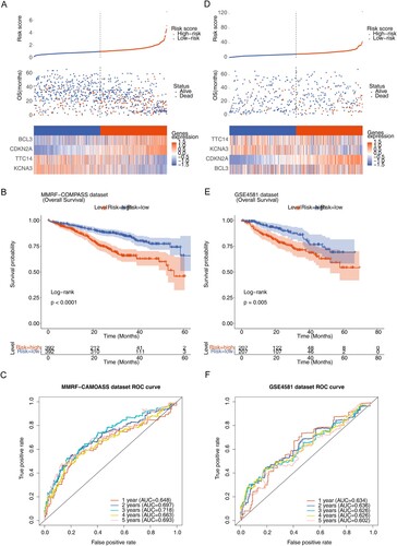
Table 3. Clinical correlation analysis between the risk score and clinical factors.
Figure 5. Independent prognostic analysis and construction of the nomogram. (A) Forest map of univariate Cox independent prognostic analysis. (B) Forest map of multivariate Cox independent prognostic analysis. (C) nomogram was constructed based on the risk model and other independent prognostic factors. (D) Calibration curve of nomogram for survival prediction at 1-, 2-, 3-years. * P < 0.05, ** P < 0.01, *** P < 0.001, **** P < 0.0001.
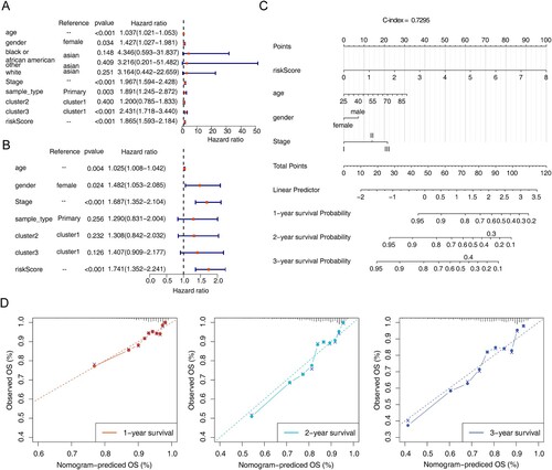
Figure 6. Gene set enrichment analysis (GSEA) for the high- and low-risk groups. (A) The activated KEGG terms in the high-risk group. (B) The activated KEGG terms in the low-risk group. (C) The enriched GO terms in the high-risk group. (D) The enriched GO terms in the low-risk group.
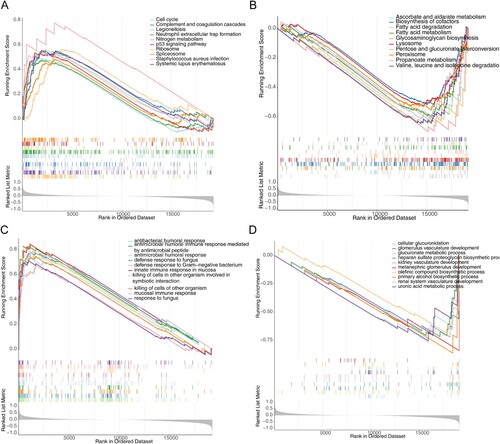
Figure 7. Immune related analyzes. (A) Box plot of stromal score, immune scores and ESTIMATE scores in high- and low-risk groups. (B) Histogram for 22 immune cells proportions in each MM patient. (C) Boxplot of the proportion of immune cells in the remaining samples. (D) Boxplot of 22 immune cells proportions in high- and low-risk groups. (E) Violin plot of cytolytic activity (CYT) levels in high- and low-risk groups. (F) Violin plot of antigen presentation mechanism (APM), tumor infiltrating lymphoid cells (TILs) and T cell infiltration relative score (TIS) in high- and low-risk groups. ns, not significant, * P < 0.05, ** P < 0.01, *** P < 0.001, **** P < 0.0001.
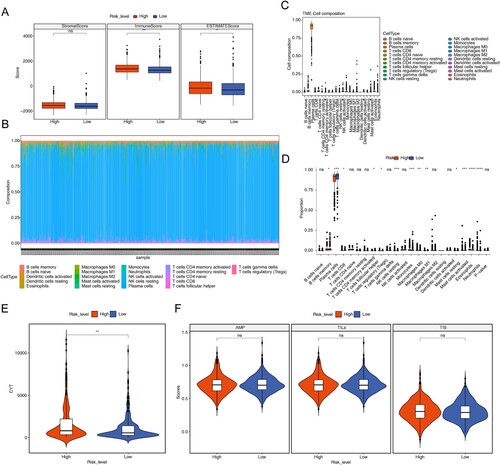
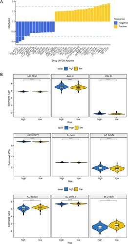
Figure 8. Potential drug prediction (A) Spearman correlation analysis between risk score and drugs from drug sensitivity in cancer (GDSc) database. (B) The 50% inhibitory concentration (IC50) of nine drugs in high- and low-risk groups. **** P < 0.0001.