New operational matrices of orthogonal Legendre polynomials and their operational

Figures & data

Figure 1. Comparing approximate solutions of Example 6.1 with the exact solutions $u_1(x,y)$ and $u_2(x,y)$ at scale level N=7.

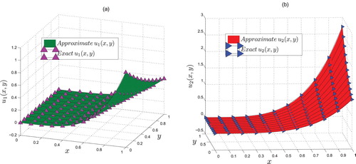
Figure 2. Comparing approximate solution with the exact solutions of Example 6.1 at fractional values of ${\eta }_1$ and ${\vartheta }_1$ at scale level N=7.

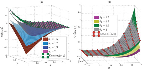
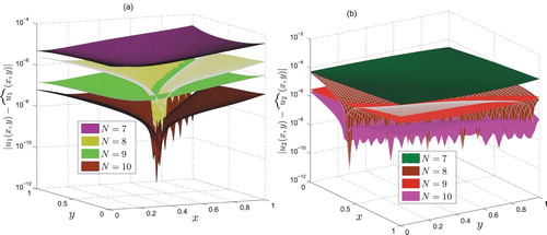
Figure 3. At different scale levels, the amount of absolute errors of Example 6.1 in $u_1(x,y)$ and $u_2(x,y)$ is noted.

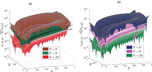
Figure 4. Comparing approximate solutions of Example 6.2 with the exact solutions $u_1(x,y)$ and $u_2(x,y)$ at scale level N=10.

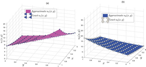
Figure 5. Comparing approximate solution with the exact solutions of Example 6.2 at fractional values of ${\eta }_1$ and ${\vartheta }_1$ at scale level N=10.

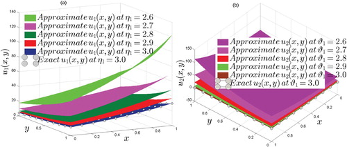
Figure 6. At scale level N=8, the amount of absolute errors of Example 6.2 in $u_1(x,y)$ and $u_2(x,y)$ is visualized.

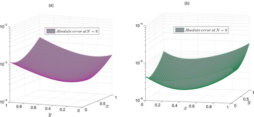
Figure 7. Comparing approximate solutions of Example 6.3 with the exact solutions $u_1(x,y)$ and $u_2(x,y)$ at scale level N=7.

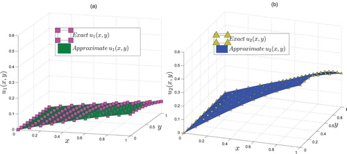
Figure 8. Comparing approximate solution with the exact solutions of Example 6.3 at fractional values of ${\eta }_1$ and ${\vartheta }_1$ at scale level N=7.

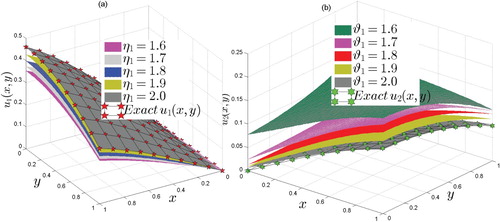
Figure 9. At different scale levels, the amount of absolute errors of Example 6.3 in $u_1(x,y)$ and $u_2(x,y)$ is visualized.