Effect of variation of charge in the circular restricted three-body problem with variable masses

Figures & data

Figure 1. Geometric configuration of the problem.

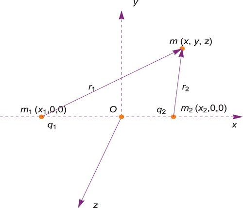
Figure 2. Locations of equilibrium points for q=0.4 (a) and for q=0.501 (b). The green points indicate the equilibrium points and red points indicate the locations of the primaries.

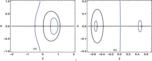
Figure 3. Zero-velocity curves $\left(a\right)$ for $q=0.4$ and $\left(b\right)$ for q=0.501.

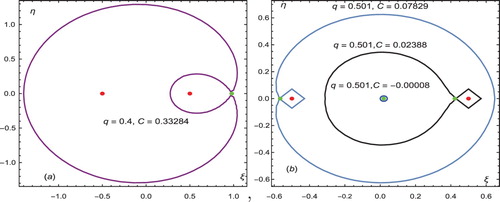
Figure 4. Epitrochoid periodic orbits for the variations of charge.

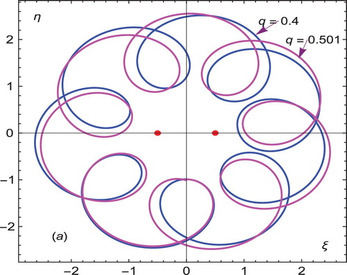
Figure 5. Zero-velocity surfaces $\left(a\right)$ for $q=0.4$ and $\left(b\right)$ for q=0.501.

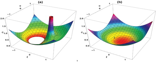
Figure 6. (a):Poincaré surfaces of section in $\xi -{\xi }^{\prime }$ plane. (b):Poincaré surfaces of section in $\eta -{\eta }^{\prime }$ plane.

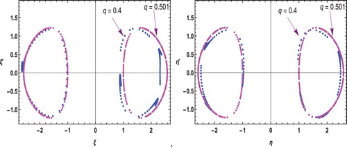
Figure 7. The surfaces of the motion of the infinitesimal body for $q=0.4$.

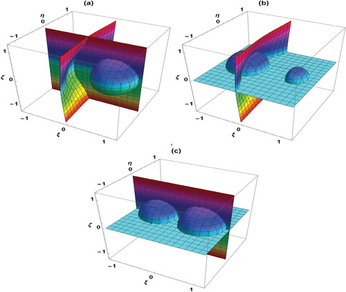
Figure 8. The surfaces of the motion of the infinitesimal body for q=0.501.

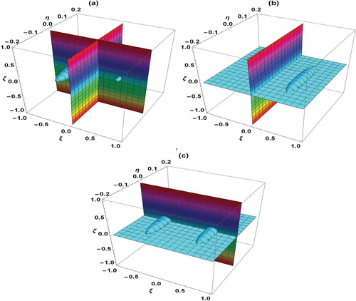
Figure 9. (a) Basins of attraction at q=0.4. (b) Zoomed part of Figure 9(a) near primaries.

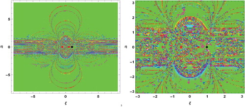
Figure 10. (a) Basins of attraction at q=0.501. (b) Zoomed part of Figure 10(a) near primaries.

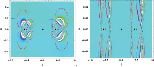
Table 1. Characteristic roots corresponding to each equilibrium point.

q	$(\xi ,\eta )$	λ
0.4	(0.9783183434, 0)	−0.6218790796, −1.2177202932 I,
		$+1.2177202932$ I, −1.6443512025 I,
		$+1.6443512025$ I, 0.6218790796
0.501	(-0.5663132332, 0)	−2.1917008069, −2.0070941992 I,
		$+2.0070941992$ I, −2.1389542543 I,
		$+2.1389542543$ I, 2.1917008069
0.501	(0.4228395029, 0)	−1.2551930819, −1.2180170977,
		−2.6189836431 I, 2.6189836431 I,
		1.2180170977, 1.2551930819
0.501	(0.0200971969, 0)	−0.2247714567 I,0.2247714567 I,
		−0.7733435483 I, +0.7733435483 I,
		−1.7752232390 I, +1.7752232390 I

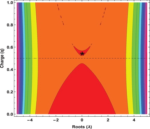
Figure 11. Distribution of the stable region.