Magnetic properties of GaAs parabolic quantum dot in the presence of donor impurity under the influence of external tilted electric and magnetic fields

Figures & data

Figure 1. Ground state energy versus no. of basis for different values of F andω₀, T = 0.1 K, θ = 60°.

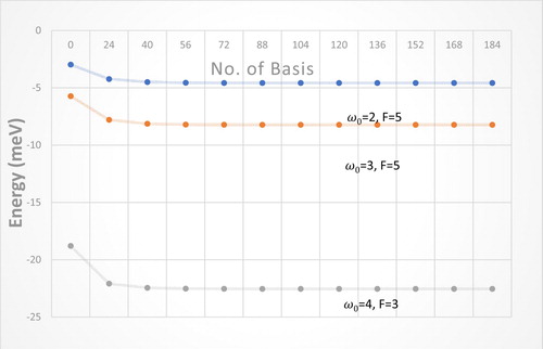
Table 1. The values of the Ground state energy and the number of basis involved in the diagonalization process, for different values of F and ω₀.

No. of basis	Ground state energy (meV)
	F = 5R*	F = 5R*	F = 3R*
No. of basis	ω0 = 2R*	ω0 = 3R*	ω0 = 4R*
0	−2.97591	−2.75044	−13.0569
24	−4.23069	−3.56145	−14.2875
40	−4.4962	−3.63935	−14.3127
56	−4.55723	−3.64566	−14.3131
72	−4.57217	−3.64607	−14.3131
88	−4.57634	−3.64609	−14.3131
104	−4.57758	−3.64609	−14.3131
120	−4.57795	−3.64609	−14.3131
136	−4.57801	−3.64609	−14.3131
152	−4.57807	−3.64609	−14.3131
168	−4.57808	−3.64609	−14.3131
184	−4.57808	−3.64609	−14.3131

Figure 2. Statistical energy against ω_c for different values of F (F = 4.8R* for solid line, = 7R* for dashed line), ω₀= 2R*, T = 0.01 K, θ = 60°.

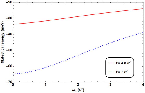
Figure 3. Statistical energy against ω_c for different values of T (T = 0.01 K for solid line, =10 K for dashed line), ω₀= 2R*, F = 4.8R*, θ = 60°.

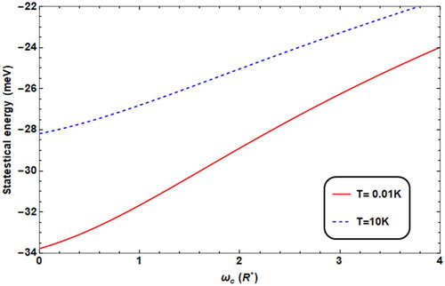
Figure 4. Statistical energy against ω_c for different values of ω₀ (ω₀ = 2R* for solid line, = 2.5R* for dashed line, = 1.5R* for dot dashed), T = 0.01 K, F = 4.8R*, θ = 60°.

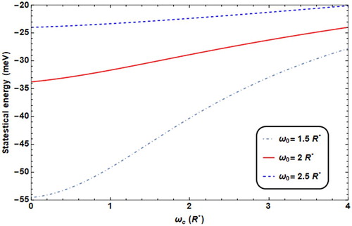
Figure 5. Statistical energy against ω_c for different values of θ (θ = 60° for solid line, =36° for thick line, = 0 for dot dashed line), ω₀= 2R*, F = 4.8R*, T = 0.01 K.

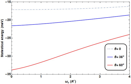
Figure 6. Statistical energy against ω_c with (dashed line)/without (solid line) impurity, ω₀= 2R*, F = 4.8 K, θ = 60°, T = 0.01 K.

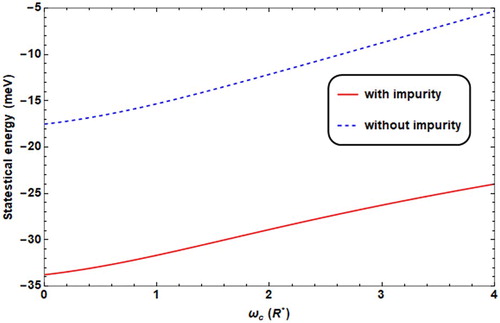
Figure 7. Magnetization versus ω_c with different F values (F = 4.8R* for solid line, = 7R* for dashed line), with ω₀= 2R*, T = 0.01 K, θ = 60°.

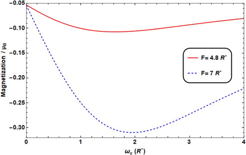
Figure 8. Susceptibility versus ω_c with different F values (F = 4.8R* for solid line, = 7R* for dashed line), with w₀= 2R*, T = 0.01 K, θ = 60°.

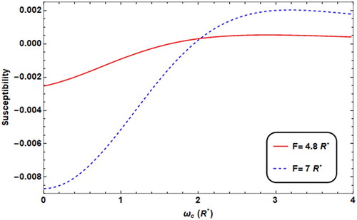
Figure 9. Magnetization versus ω_c with different T values (T = 0.01 K for solid line, = 10K* for dashed line) with ω₀= 2R*, F = 4.8R*, θ = 60°.

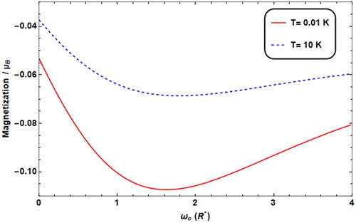
Figure 10. Susceptibility versus ω_c with different T values (T = 0.01 K for solid line, = 10K* for dashed line) with ω₀= 2R*, F = 4.8R*, θ = 60°.

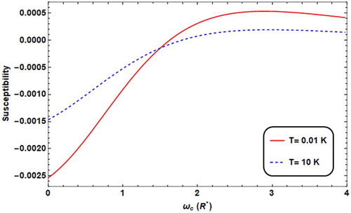
Figure 11. Magnetization versus ω_c with different ω₀ values (ω₀= 2R* for solid line, = 2.5R* for dashed line, = 1.5R* for dot dashed) with T = 0.01 K, F = 4.8R*, θ = 60°.

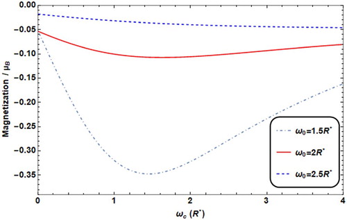
Figure 12. Susceptibility versus ω_c with different ω₀ values (ω₀= 2R* for solid line, = 2.5R* for dashed line, = 1.5R* for dot dashed) with T = 0.01 K, F = 4.8R*, θ = 60°.

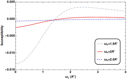
Figure 13. Magnetization versus ω_c with different θ values (θ = 60° for solid line, = 36° for thick line, = 0° for dot dashed) with T = 0.01 K, F = 4.8R*, ω₀ = 2R*.

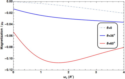
Figure 14. Susceptibility versus ω_c with different θ values (θ = 60° for solid line, = 36° for thick line, = 0° for dot dashed) with T = 0.01 K, F = 4.8R*, ω₀ = 2R*.

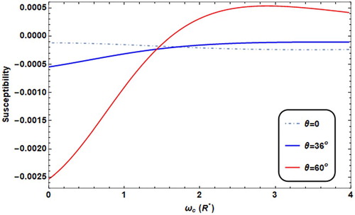
Figure 15. Magnetization versus ω_c with the presence/absence of impurity (solid/dashed) with T = 0.01 K, F = 4.8R*, ω₀ = 2R*, θ = 60°.

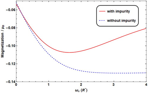
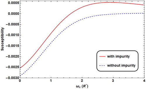
Figure 16. Susceptibility versus ω_c with the presence/absence of impurity (solid/dashed) with T = 0.01 K, F = 4.8R*, ω₀= 2R*, θ = 60°.