Evaluation of the anticorrosion performance of Tamsulosin as corrosion inhibitor for pipeline steel in acidic environment: experimental and theoretical study

Figures & data

Figure 1. (a) Molecular and (b) 3D ball and stick structures of TAM.

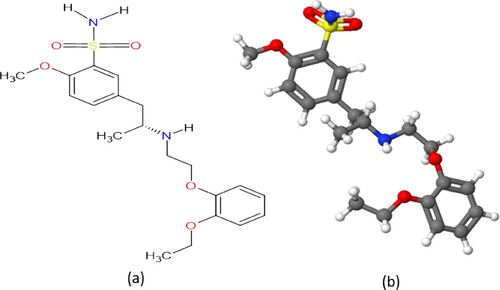
Table 1. Comparison of the inhibitive performance of TAM with other reported drug corrosion inhibitors.

Drug name	Metal and electrolyte	Inhibitor concentration	Inhibition efficiency, %	Reference
Tramadol	Aluminium in 1 M HCl	500 ppm	96	[11]
Chloraphenicol	Mild steel in 0.1 M HCl	10% v/v	85	[12]
Cephapirin	Carbon steel in 2M HCl	600 ppm	83	[13]
Chemically modified Dapsone	Mild steel in 0.5 M H2SO4	0.219 nM	95	[14]
Irbesartan	Mild steel in 0.5 M H2SO4	300 mg/L	83	[15]
Dexamethasone	Mild steel in 2 M HCl	0.4 g/L	83	[16]
Ranitidine	Aluminium in 1 M HCl	400 ppm	90	[17]
Cefixime	Mild steel in 1 M HCl	8.8 × 10^−4 M	62	[18]
Cefazolin	Mild steel in 1 M HCl	11 × 10^−4 M	68	[19]
Methocarbamol	Mild steel in 2.5 M H2SO4	2 × 10^−3 M	67	[20]
TAM	St52 steel in 1 M HCl	2.0 × 10^−3 M	94	This work

Figure 2. Variation of (a) $C_R$ and (b) ${\eta }_{WL}\mathrm{\%}$ of TAM with inhibitor concentration in 1 M HCl at various temperatures.

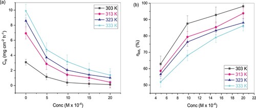
Figure 3. Plot of $\log C_R$ versus $1/T$ for St52 steel corrosion in 1M HCl and inhibited solutions at various concentrations of TAM.

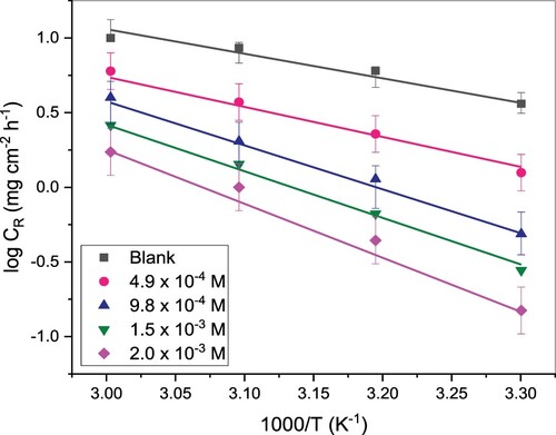
Figure 4. Plot of $\log C_R/T$ versus $1/T$ for corrosion of St52 steel in 1 M HCl and solution and inhibited solutions at different concentrations of TAM.

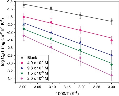
Table 2. Computed ${\text{E}}_{\text{a}}$ values and thermodynamics parameters for St52 steel corrosion in 1 M HCl solution without and with various TAM concentrations.

Conc. (M)	${\text{E}}_{\text{a}}(\text{kJ}/\text{mol})$	$\mathrm{\Delta }{\text{H}}^{\ast }(\text{kJ}/\text{mol})$	$\mathrm{\Delta }{\text{S}}^{\ast }(\text{J}/\text{mol}/\text{K})$
Blank	31.32	26.69	−146.19
4.9 × 10^−4	36.71	29.05	−141.83
9.8 × 10^−4	40.90	34.73	−136.05
1.5 × 10^−3	43.74	36.64	−131.62
2.0 × 10^−3	45.92	40.88	−127.81

Figure 5. (a) Nyquist, (b) phase angle and (c) Bode modulus plots of St52 steel in 1M HCl without and in different concentrations of TAM.

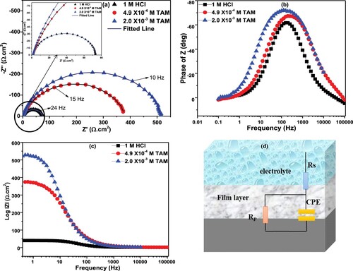
Table 3. Impedance data for St52 steel in 1M HCl and with various concentrations TAM at 303 K.

Conc. (M)	$R_s$ (Ω cm^2)	$R_{ct}$ (Ω cm^2)	$Q$ (μΩ^−1 s^n cm^−2)	$C_{dl}$ (μF cm^−2)	$n$	${\eta }_{EIS}$ (%)
Blank	1.17	60	189.3	130.4	0.88	—
4.9 × 10^−4	0.94	372.5	160.1	86.6	0.89	83
2.0 × 10^−3	1.25	519.6	90.2	10.3	0.89	88

Figure 6. (a) Open circuit potential and (b) polarization curves of St52 steel in1 M HCl and in the presence of different TAM concentrations.

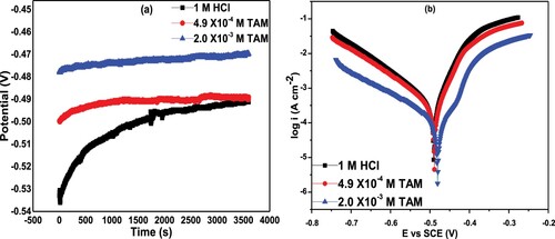
Figure 7. SEM/EDX images of St52 steel surface in (a) 1 M HCl without and (b) with 2.0 × 10⁻³ M of TAM.

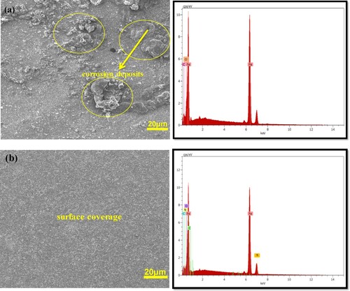
Table 4. Polarization data for St52 steel corrosion in 1.5 M HCl in the absence and presence of TAM.

Concentration (M)	$-E_{corr}$ (mV/SCE)	$i_{corr}$ (µA cm^−2)	${\beta }_a$ (mV dec^−1)	−${\beta }_c$ (mV dec^−1)	${\eta }_{PDP}$ (%)
Blank	−503.4	182.4	120.2	130.5	—
4.9 × 10^−4	−500.2	26.2	110.4	127.3	85.6
2.0 × 10^−3	−491.6	10.8.	82.8	128.6	94.1

Figure 8. Langmuir isotherm plots for TAM’s adsorption on St52 steel surface at various temperatures.

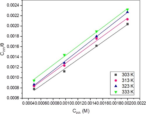
Table 5. Langmuir adsorption isotherm data for TAM at various temperatures.

Temp. (K)	Intercept	Slope	$R^2$	$K_{ads}$ (M^−1)	$\mathrm{\Delta }{G}_{ads}$ (kJ/mol)
303	3.36 × 10^−4	0.8472	0.9967	2976	−30.27
313	4.04 × 10^−4	0.8741	0.9969	2475	−30.79
323	4.51 × 10^−4	0.9368	0.9992	2217	−31.47
333	5.23 × 10^−4	0.9073	0.9982	1912	−32.04

Figure 9. Spatial adsorption interactions of TAM on St52 steel surface.

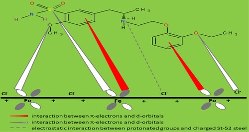
Figure 10. Systematic and staggered arrangement of TAM on St52 steel surface.

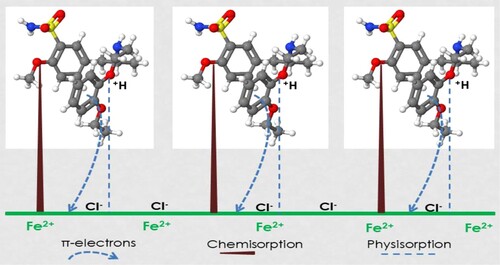
Figure 11. The FMO density distribution of HOMO and LUMO of neutral and protonated TAM.

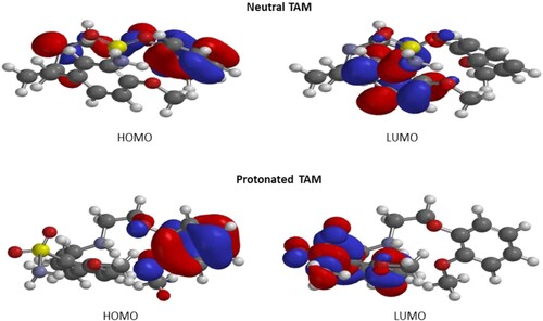
Table 6. DFT parameters for neutral (TAM) and protonated (TAM-H⁺) form of the inhibitor.

Inhibitor	$E_{HOMO}$ (eV)	$E_{LUMO}$ (eV)	$\mathrm{\Delta }{E}_{gap}$ (eV)	$\chi$ (eV)	$\eta$ (eV)	$\sigma$ (eV^−1)	$\mathrm{\Delta }N$	$\mu$ (Debye)	Total energy (au)
TAM	−5.37	−0.87	4.50	3.12	2.25	0.44	0.86	7.27	−1622
TAM-H^+	−11.05	−8.24	2.81	3.65	1.41	0.71	1.19	10.22	−1624

Abdallah M, Gad EAM, Sobhi M, et al. Performance of tramadol drug as a safe inhibitor for aluminum corrosion in 1.0 M HCl solution and understanding mechanism of inhibition using DFT. Egypt. J. Pet. 2019;28:173–181.

 Google Scholar

Ayoola AA, Fayomi OSI, Ogunkanmbi SO. Data on inhibitive performance of chloraphenicol drug on A315 mild steel in acidic medium. Data Br. 2018;19:804–809.

 PubMed Web of Science ®Google Scholar

EL-Haddad ME, Fouda AS, Hassan AF. Data from chemical, electrochemical and quantum chemical studies for interaction between Cephapirin drug as an eco-friendly corrosion inhibitor and carbon steel surface in acidic medium. Chem. Data Collect. 2019;22:100251.

 Google Scholar

Singh P, Chauhan DS, Chauhan SS, et al. Chemically modified expired Dapsone drug as environmentally benign corrosion inhibitor for mild steel in sulphuric acid useful for industrial pickling process. J Mol Liq. 2019;286:110903.

 Web of Science ®Google Scholar

Srivastava M, Tiwari P, Srivastava SK, et al. Electrochemical investigation of Irbesartan drug molecules as an inhibitor of mild steel corrosion in 1M HCl and 0.5 M H2SO4 solutions. J Mol. Liq. 2017;236:184–197.

 Web of Science ®Google Scholar

Anadebe VC, Onukwuli OD, Abeng FE, et al. Electrochemical-kinetics, MD-simulation and multi-input single-output (MISO) modeling using adaptive neuro-fuzzy inference system (ANFIS) prediction for dexamethasone drug as eco-friendly corrosion inhibitor for mild steel in 2M HCl electrolyte. J Taiwan Inst. Chem. Eng. 2020;115:251–265.

 PubMed Web of Science ®Google Scholar

Hameed RS A. Expired Ranitidine drugs as corrosion inhibitor for aluminum in 1M HCl. Al-Azhar Bull Sci. 2009;20:151–163.

 Google Scholar

Naqvi I, Saleemi AR, Naveed S. Cefixime: A drug as efficient corrosion inhibitor for mild steel in Acidic Media: electrochemical and thermodynamic studies. Int J Electrochem Sci. 2011;6:146–161.

 Web of Science ®Google Scholar

Singh AK, Quraishi MA. Effect of Cefazolin on the corrosion of mild steel in HCl solution. Corros. Sci. 2010;52:152–160.

 Web of Science ®Google Scholar

Ebenso EE, Eddy NO, Odiongenyi AO. Corrosion inhibition and adsorption properties of Methocarbamol on mild steel in acidic medium. Port. Electrochim. Acta. 2009;27:13–22.

 Google Scholar