Numerical study of multi-order fractional differential equations with constant and variable coefficients

Figures & data

Figure 1. The maximum absolute errors determined by our method are compared with the maximum absolute errors determined by the method ([22], Example 2, n = 3. (a) (Our proposed method) and (b) (Proposed method in [22])).

Table 1. Maximum absolute error of Example 7.5 at $n=\{2,3,4,6\}$=scale level=number of terms of SLPs, and for different values of t.

t	n = 2	n = 3	n = 4	n = 6
0.0	0.0000	0.0000	0.0000	$4.5537\times {10}^{-41}$
0.2	$2.3616\times {10}^{-3}$	$6.7672\times {10}^{-4}$	$1.1310\times {10}^{-4}$	$5.4764\times {10}^{-5}$
0.4	$3.2289\times {10}^{-3}$	$1.7558\times {10}^{-4}$	$2.3608\times {10}^{-4}$	$5.0444\times {10}^{-5}$
0.6	$2.6020\times {10}^{-3}$	$5.7017\times {10}^{-4}$	$1.0341\times {10}^{-4}$	$7.8996\times {10}^{-6}$
0.8	$4.8096\times {10}^{-4}$	$6.2728\times {10}^{-4}$	$3.2997\times {10}^{-4}$	$4.8405\times {10}^{-5}$
1.0	$3.1343\times {10}^{-3}$	$9.3751\times {10}^{-4}$	$2.4238\times {10}^{-4}$	$4.7670\times {10}^{-5}$

Table 2. Legendre series coefficients ($e_{10},e_{11},e_{12},e_{13}$) for Example 7.2 obtained by using our proposed method (PM) and the Jacobi series coefficients ($e_{10}=c_0,e_{11}=c_1,e_{12}=c_2,e_{13}=c_3$) obtained by using the method ([19], Example 4), when $\alpha =\beta =0$, and n = 3= scale level= the number of terms of SLPs.

Coefficients	PM	Method proposed in [19]
$e_{10}$	$\frac{1}{3}$	$\frac{1}{3}$
$e_{11}$	$\frac{1}{2}$	$\frac{1}{2}$
$e_{12}$	$\frac{1}{6}$	$\frac{1}{6}$
$e_{13}$	$5.2456\times {10}^{-37}$	0

Table 3. Comparison of approximate solution (AS) for Example 7.2 obtained by using our proposed method (PM) and the AS obtained by using the method ([19], Example 4), when $\alpha =\beta =0$, and n = 3=scale level=number of terms of SLPs.

t	Exact solution	AS using PM	AS using the method [19]
0	0	$-1.4694\times {10}^{-39}$	0
0.1	0.01	0.01	0.01
0.2	0.04	0.04	0.04
0.3	0.09	0.09	0.09
0.4	0.16	0.16	0.16
0.5	0.25	0.25	0.25
0.6	0.36	0.36	0.36
0.7	0.49	0.49	0.49
0.8	0.64	0.64	0.64
0.9	0.81	0.81	0.81
1.0	1.0	1.0	1.0

Table 4. AE for Example 7.2 computed by using our proposed method (PM) and the AE computed by using the method ([19], Example 4), when $\alpha =\beta =0$, and n = 3=scale level=number of terms of SLPs.

t	Exact solution	AE using PM	AE using the method [19]
0	0	$1.4694\times {10}^{-39}$	0
0.1	0.01	0	0
0.2	0.04	0	0
0.3	0.09	0	0
0.4	0.16	0	0
0.5	0.25	0	0
0.6	0.36	0	0
0.7	0.49	0	0
0.8	0.64	0	0
0.9	0.81	0	0
1.0	1.0	0	0

Figure 2. Exact and the approximate solutions of Example 7.3 are compared at different scale levels.

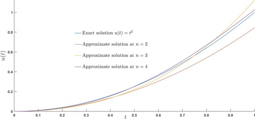
Figure 3. Error plots of Example 7.3 at different scale levels.

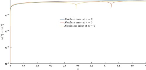
Figure 4. Exact and the approximate solutions of Example (7.4) are compared at various values of ${\beta }_1$.

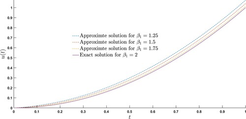
Figure 5. Exact and the approximate solutions of Example (7.5) are compared at different scale levels.

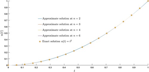
Figure 6. Exact and the approximate solutions of Example 7.2 are compared at n = 4, ${\beta }_1=3$, and ${\beta }_2=2.5$.

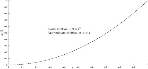
Table 5. Maximum absolute error of Example 7.4 at n = 10=scale level=number of terms of SLPs and for various choices of ${\beta }_1$.

t	${\beta }_1=1.25$	${\beta }_1=1.5$	${\beta }_1=1.75$	${\beta }_1=2$
0.0	$1.83\times {10}^{-40}$	$9.18\times {10}^{-41}$	$1.83\times {10}^{-40}$	0
0.2	$2.25\times {10}^{-2}$	$1.35\times {10}^{-2}$	$5.58\times {10}^{-3}$	0
0.4	$4.13\times {10}^{-2}$	$2.44\times {10}^{-2}$	$9.70\times {10}^{-3}$	0
0.6	$5.63\times {10}^{-2}$	$3.26\times {10}^{-2}$	$1.23\times {10}^{-2}$	0
0.8	$6.74\times {10}^{-2}$	$3.81\times {10}^{-2}$	$1.35\times {10}^{-2}$	0
1.0	$7.48\times {10}^{-2}$	$4.08\times {10}^{-2}$	$1.32\times {10}^{-2}$	0

Table 6. The Approximate solution of Example 7.5 is calculated at $n=\{2,3,4,6\}$=scale level=number of terms of SLPs, and for different values of t.

t	n = 2	n = 3	n = 4	n = 6
0.0	0.0000	0.0000	0.0000	0.0000
0.2	0.0424	0.0407	0.0401	0.0399
0.4	0.1632	0.1602	0.1598	0.1601
0.6	0.3626	0.3594	0.3599	0.3600
0.8	0.6405	0.6394	0.6403	0.6400
1.0	0.9969	1.0009	0.9998	1.0000

Table 7. Absolute error (AE) of Example 7.2 at $n=\{3,4\}$ = scale level= the number of terms of SLPs.

t	Exact solution	AE at n = 3	AE at n = 4
0	0	$1.4694\times {10}^{-39}$	$1.1615\times {10}^{-40}$
0.2	0.04	0	0
0.4	0.16	0	0
0.6	0.36	0	0
0.8	0.64	0	0
1.0	1.0	0	0

Pak S, Choi H, Sin K, et al. Analytical solutions of linear inhomogeneous fractional differential equation with continuous variable coefficients. Adv Differ Equ. 2019;2019(256):1–22.

 Google Scholar

Doha E, Bhrawy A, Ezz-Eldien S. A new Jacobi operational matrix: an application for solving fractional differential equations. Appl Math Model. 2012;36(10):4931–4943.

 Web of Science ®Google Scholar