1,764
Views
68
CrossRef citations to date
0
Altmetric
Research Article

Dynamic study of multi-peak solitons and other wave solutions of new coupled KdV and new coupled Zakharov–Kuznetsov systems with their stability

, , , &
Article: 2163872 | Received 24 Nov 2022, Accepted 26 Dec 2022, Published online: 20 Feb 2023

Figures & data

Figure 1. Appropriate parameter values to result (Equation19) are illustrated as follows: Figures (A,B,E) describe the bright soliton and their 2D contour plot figures (B,D,F), respectively, at δ=1,γ=0.5,β=1.5,A1=1.5,A2=0.1,σ=1,λ=1,α=0,a0=1.

Figure 1. Appropriate parameter values to result (Equation19(19) u1(ξ)=a0+6βδ2σ(A2sinh⁡(ξ−σ)+A1cosh⁡(ξ−σ))2λ(A1sinh⁡(ξ−σ)+A2cosh⁡(ξ−σ))2,v1(ξ)=βδ2(α2+4γλ−α)(a0βδ2+6σ(A2sinh⁡(ξ−σ)+A1cosh⁡(ξ−σ))2λ(A1sinh⁡(ξ−σ)+A2cosh⁡(ξ−σ))2)2γ,w1(ξ)=βδ2(α2+4γλ−α)(a0βδ2+6σ(A2sinh⁡(ξ−σ)+A1cosh⁡(ξ−σ))2λ(A1sinh⁡(ξ−σ)+A2cosh⁡(ξ−σ))2)2γ.(19) ) are illustrated as follows: Figures (A,B,E) describe the bright soliton and their 2D contour plot figures (B,D,F), respectively, at δ=1,γ=0.5,β=1.5,A1=1.5,A2=0.1,σ=−1,λ=1,α=0,a0=1.

Figure 2. Appropriate parameter values to result (Equation20) are depicted as follows: Figures (A,C,E) are multi-peak solitons with various amplitudes and their 2D contourplots in figures (B,D,F) respectively, at δ=1,γ=0.75,β=0.5,A1=0.5,A2=0.1,σ=0.5,λ=1.

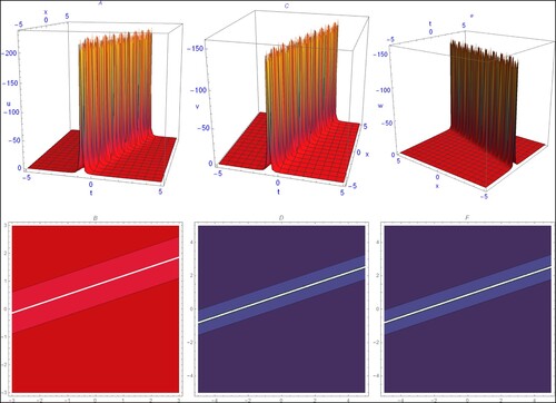
Figure 2. Appropriate parameter values to result (Equation20(20) u2(ξ)=6βδ2σ(A12−A22)λ(A1sinh⁡(ξ−σ)+A2cosh⁡(ξ−σ))2,v2(ξ)=3σβδ2(A12−A22)(α2+4γλ−α)γλ(A1sinh⁡(ξ−σ)+A2cosh⁡(ξ−σ))2,w2(ξ)=3σβδ2(A12−A22)(α2+4γλ−α)γλ(A1sinh⁡(ξ−σ)+A2cosh⁡(ξ−σ))2.(20) ) are depicted as follows: Figures (A,C,E) are multi-peak solitons with various amplitudes and their 2D contourplots in figures (B,D,F) respectively, at δ=1,γ=0.75,β=0.5,A1=0.5,A2=0.1,σ=−0.5,λ=1.

Figure 3. Appropriate parameter values to the result (Equation21) are depicted as follows: Figures (A,C,E) are periodic solitons with various amplitudes and their 2D contourplots in figures (B,D,F), respectively, at δ=1,γ=2,β=3,A1=1.5,A2=0.1,σ=1,λ=1,α=0,a0=1.

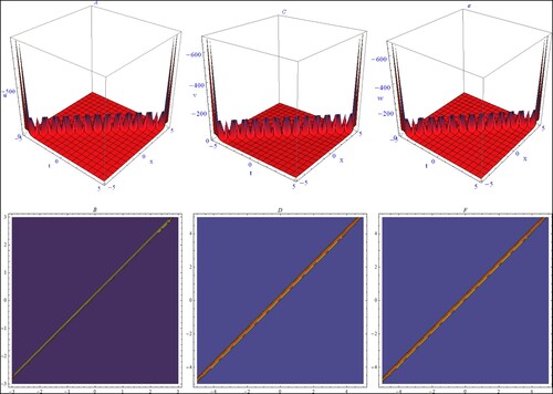
Figure 3. Appropriate parameter values to the result (Equation21(21) u3(ξ)=a0−6βδ2σ(A1cos⁡(ξσ)−A2sin⁡(ξσ))2λ(A1sin⁡(ξσ)+A2cos⁡(ξσ))2,v3(ξ)=βδ2(α2+4γλ−α)(a0βδ2−6σ(A1cos⁡(ξσ)−A2sin⁡(ξσ))2λ(A1sin⁡(ξσ)+A2cos⁡(ξσ))2)2γ,w3(ξ)=βδ2(α2+4γλ−α)(a0βδ2−6σ(A1cos⁡(ξσ)−A2sin⁡(ξσ))2λ(A1sin⁡(ξσ)+A2cos⁡(ξσ))2)2γ.(21) ) are depicted as follows: Figures (A,C,E) are periodic solitons with various amplitudes and their 2D contourplots in figures (B,D,F), respectively, at δ=1,γ=2,β=3,A1=1.5,A2=0.1,σ=1,λ=1,α=0,a0=1.

Figure 4. Appropriate parameter values to the result (Equation30) are followed as follows: Figures (A,C,E) are the solitons of multi-peak and their 2D contourplot in figures (B,D,F), respectively, at δ=0.3,γ=0.8,β=1,A1=0.5,A2=0.1,σ=0.1,λ=1,α=0,a0=1,y=0.1,ν=1.

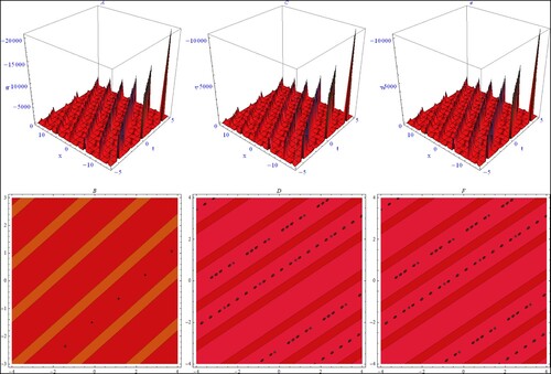
Figure 4. Appropriate parameter values to the result (Equation30(30) u2(ξ)=2βσ(δ2−ν2)(2A2A1sinh⁡(2ξ−σ)+A12(cosh⁡(2ξ−σ)+2)+A22(cosh⁡(2ξ−σ)−2))λ(A1sinh⁡(ξ−σ)+A2cosh⁡(ξ−σ))2,v2(ξ)=−σ(2A2A1sinh⁡(2ξ−σ)+A12(cosh⁡(2ξ−σ)+2)+A22(cosh⁡(2ξ−σ)−2))(β2(δ2−ν2)2(α2+4γλ)+αβ(δ2−ν2))γλ(A1sinh⁡(ξ−σ)+A2cosh⁡(ξ−σ))2,w2(ξ)=−σ(2A2A1sinh⁡(2ξ−σ)+A12(cosh⁡(2ξ−σ)+2)+A22(cosh⁡(2ξ−σ)−2))(β2(δ2−ν2)2(α2+4γλ)+αβ(δ2−ν2))γλ(A1sinh⁡(ξ−σ)+A2cosh⁡(ξ−σ))2.(30) ) are followed as follows: Figures (A,C,E) are the solitons of multi-peak and their 2D contourplot in figures (B,D,F), respectively, at δ=0.3,γ=0.8,β=1,A1=0.5,A2=0.1,σ=−0.1,λ=1,α=0,a0=1,y=0.1,ν=1.

Figure 5. Appropriate parameter values to result (Equation32) are illustrated as follows: Figures (A,C,E) are periodic solitons with dissimilar amplitude and their 2D Contourplots in figures (B,D,F) respectively, at δ=0.3,γ=0.8,β=1,A1=0.5,A2=0.1,σ=0.1,λ=1,a0=1,y=0.1,ν=1.

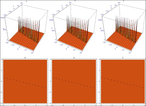
Figure 5. Appropriate parameter values to result (Equation32(32) u4(ξ)=2β(ν2−δ2)(3σ(A1cos⁡(ξσ)−A2sin⁡(ξσ))2(A1sin⁡(ξσ)+A2cos⁡(ξσ))2+σ)λ,v4(ξ)=σ(−2A2A1sin⁡(2ξσ)+A12(cos⁡(2ξσ)+2)−A22(cos⁡(2ξσ)−2))(β2(δ2−ν2)2(α2+4γλ)+αβ(δ2−ν2))γλ(A1sin⁡(ξσ)+A2cos⁡(ξσ))2,w4(ξ)=σ(−2A2A1sin⁡(2ξσ)+A12(cos⁡(2ξσ)+2)−A22(cos⁡(2ξσ)−2))(β2(δ2−ν2)2(α2+4γλ)+αβ(δ2−ν2))γλ(A1sin⁡(ξσ)+A2cos⁡(ξσ))2.(32) ) are illustrated as follows: Figures (A,C,E) are periodic solitons with dissimilar amplitude and their 2D Contourplots in figures (B,D,F) respectively, at δ=0.3,γ=0.8,β=1,A1=0.5,A2=0.1,σ=−0.1,λ=1,a0=1,y=0.1,ν=1.

Figure 6. The DR between frequency(ω) and wave number (k) of (Equation38) is shown in (A) and DR between frequency(ν) and wave numbers (ω1,ω2) of (Equation43) is shown in (B).

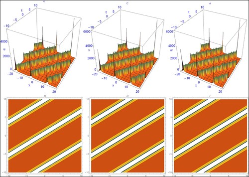
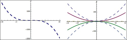
Figure 6. The DR between frequency(ω) and wave number (k) of (Equation38(38) ω=12(2δPϵ−2βk3−αkP−λkP±k2P(α2+2αλ+8γλ+λ2)).(38) ) is shown in (A) and DR between frequency(ν) and wave numbers (ω1,ω2) of (Equation43(43) ν=12(−2βσ13−2βσ22σ1−αPσ1+2δPϵ−λPσ1±α2Pσ12+2αλPσ12+8γλPσ12+λ2Pσ12).(43) ) is shown in (B).