Comparative molecular dynamics simulation of apo and holo forms of the P53 mutant C176F: a structural perspective

Figures & data

Figure 1. The WT P53 protein in apo and holo forms were visualized using BIOVIA Discovery Studio Visualizer (A) Apo form of P53 protein, (B) Holo form of P53 protein. The distance between the Zn2 + ion and the binding residues are represented.

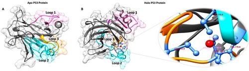
Figure 2. Various cancer types with C176 mutation samples (A) Data reported by a database of Catalogue Of Somatic Mutations In Cancer (COSMIC) and (B) TCGA cancer report.

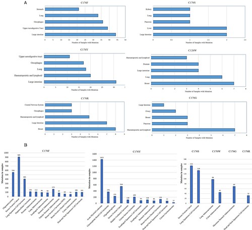
Table 1. Prediction of stability change by DDG for the variant C176F.

Tools	DDG kcal/mol	Stability
i-Mutant2.0 SEQ	−1.61	Decrease
MUpro	−1.04	Decrease
PremPS	0.98	Decrease
INPS-MD	−2.76	Decrease
CUPSAT	−1.5	Destabilizing
DynaMut 2	−0.99	Destabilizing
iStable	0.604838	Decrease

Figure 3. The Backbone Root Mean Square Deviation (RMSD) and value for WT and MT C176F of P53 protein in Apo and Holo simulations at 500 ns (A) Apo WT (Grey), Apo MT (red), (B) Holo WT (Grey), Holo MT (Blue). The Root Mean Square Fluctuation (RMSF) of Cα atoms for WT and MTC176F of P53 protein in Apo and Holo simulations at 500 ns (C) Apo WT (Grey), Apo MT (red), (D) Holo WT (Grey), Holo MT (Blue).

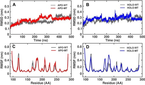
Table 2. The average value of time of structural properties for RMSD, Cα-RMSF, Rg, and SASA are calculated for WT and MT of Apo and Holo-structure of P53 protein.

	Apo		Holo
	WT	MT	WT	MT
Backbone RMSD (nm)	0.25	0.28	0.26	0.28
Cα-RMSF (nm)	0.43755	0.6329	0.4926	0.50905
Rg (nm)	1.665488957	1.673102703	1.66618413	1.680861024
SASA (nm^2)	108.003	108.859	108.889	109.114
Trace of the covariance matrix diagonalized (nm^2)	5.60441	6.59661	5.35048	7.08271

Figure 4. Radius of gyration (Rg), for Apo and Holo P53 protein simulations for WT and MT at 500 ns (A) Apo simulations for WT and MT C176F, (B) Holo simulation for WT and MT C176F, and Solvent Accessible Surface Area (SASA) during 500 ns representing Apo and Holo simulation versus time, (C) SASA of Apo WT and MT C176F, and (D) SASA of Holo WT and MT C176F.

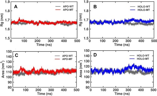
Figure 5. The Kernel Density Estimation (KDE) correlation plot of Rg and SASA. (A) Apo WT, (B) Apo MT, (C) Holo WT, and (D) Holo MT. The probability distribution is shown by concentric circles that are differentiated by the intensity.

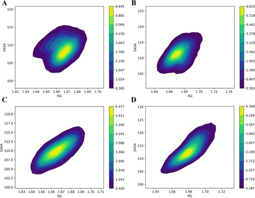
Figure 6. Dynamic Cross-correlation matrix (DCCM) of backbone atoms. (A) Apo WT, (B) Apo MT, (C) Holo WT, and (D) Holo MT. DCCM maps were obtained from 500 ns trajectories that contain contours of different colours. Correlated motion and anti-correlated motions are represented by reddish-orange and dark blue contours, respectively. The square shape represents residue motion and the circle and ellipse shapes resemble loop 1 and loop 2 regions respectively.

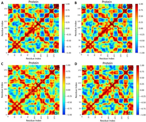
Figure 7. Gibbs free energy landscape of PC1 & PC2 (initial two principal components) of projection of simulated trajectories. (A) Apo WT, (B) Apo MT, (C) Holo WT, and (D) Holo MT obtained during 500 ns MD simulation.

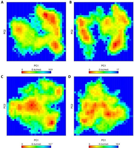
Figure 8. Principal Component Analysis of the first two eigenvectors (A) Apo WT (black) and MT structure (red), (B) Holo WT (mint green) and MT (orange) structures and (C) eigenvalues for the first 40 modes of motion.

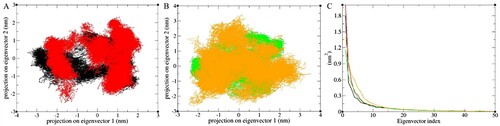
Table 3. The average percentage of secondary structure values from trajectory analysis of 500 ns for WT and MT of Apo and Holo P53 protein.

	Type	Structure (%)	α-Helix (%)	β-Sheet (%)	Coils (%)	Bends (%)	Turns (%)
Apo	WT	54	6	32	31	15	13
	MT	53	5	34	29	15	14
Holo	WT	54	5	33	29	15	15
	MT	50	5	33	33	15	11

Figure 9. The flexibility of the loops was analyzed by angle calculation using the software Maestro v 2021. (A) Apo WT, (B) Apo MT, (C) Holo WT, and (D) Holo MT Colour representation as follows: Loop 1 (dark orange in colour), Loop 2 (dark green in colour), and Loop 3 (dark pink in colour) during 0 ns (Grey in colour), and Loop 1 (light orange in colour), Loop 2 (light green in colour), and Loop 3 (light pink in colour) during 500 ns (Blue in colour) of MD simulation.

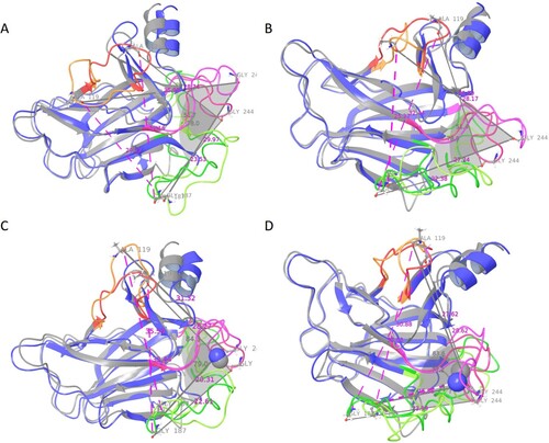
Table 4. The calculation of angles and distances for L1, L2, and L3 was conducted using the 2021 version of Maestro from Schrodinger.

Protein Type	Apo WT		Apo MT		Holo WT		Holo MT
Simulation Period	0 ns	500 ns	0 ns	500 ns	0 ns	500 ns	0 ns	500 ns
Angle	78.0°	51.7°	78.9°	51.4°	79.0°	84.3°	77.2°	83.6°
L1 (ALA 119) to L2 (GLY 244)	28.74 Å	35.95 Å	30.59 Å	28.17 Å	28.27 Å	31.32 Å	28.62 Å	27.62 Å
L2 (GLY 244) to L3 (GLY 187)	23.53 Å	29.97 Å	22.38 Å	27.24 Å	22.61 Å	20.31 Å	23.99 Å	15.86 Å
L3 (GLY 187) to L1 (ALA 119)	33.16 Å	29.22 Å	32.44 Å	25.27 Å	32.64 Å	35.59 Å	33.03 Å	30.88 Å