605
Views
5
CrossRef citations to date
0
Altmetric
Articles

Improved simulation of the East Asian winter monsoon interannual variation by IAP/LASG AGCMs

, , , &
Pages 204-210 | Received 28 Dec 2015, Accepted 20 Jan 2016, Published online: 08 Mar 2016

Figures & data

Figure 1. Climatology of 1000-hPa winds (vectors; m s−1), SLP (contours; hPa), and 2-m temperature (shading; °C) in winter (December–January–February), derived from (a) the observation (NCEP-2), (b) GAMIL1, and (c) GAMIL2. (d) Taylor diagram: The observation is considered as the reference (REF); the angular (vertical) coordinate is the pattern correlation coefficient (ratio of standard deviation) between the model and observation. The nearer the distance between a number and REF, the better the performance of the corresponding model.
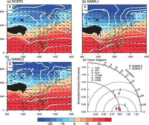
Figure 1. Climatology of 1000-hPa winds (vectors; m s−1), SLP (contours; hPa), and 2-m temperature (shading; °C) in winter (December–January–February), derived from (a) the observation (NCEP-2), (b) GAMIL1, and (c) GAMIL2. (d) Taylor diagram: The observation is considered as the reference (REF); the angular (vertical) coordinate is the pattern correlation coefficient (ratio of standard deviation) between the model and observation. The nearer the distance between a number and REF, the better the performance of the corresponding model.

Figure 2. (a) Normalized EAWM index (1000-hPa meridional wind averaged within the box (10–30°N, 115–130°E)) derived from the observation (NCEP-2; black line), GAMIL1 (red line), and GAMIL2 (blue line). Green line: normalized (−1) × Niño3.4 index. (b–e) Regression coefficients of the December–January–February 1000-hPa winds (vectors; m s−1) and precipitation (shaded; mm d−1) with respect to the EAWM index derived from (b) the observation (NCEP-2), (c) GAMIL1, (d) GAMIL2, and (e) the difference between GAMIL2 and GAMIL1.
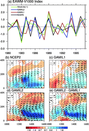
Figure 2. (a) Normalized EAWM index (1000-hPa meridional wind averaged within the box (10–30°N, 115–130°E)) derived from the observation (NCEP-2; black line), GAMIL1 (red line), and GAMIL2 (blue line). Green line: normalized (−1) × Niño3.4 index. (b–e) Regression coefficients of the December–January–February 1000-hPa winds (vectors; m s−1) and precipitation (shaded; mm d−1) with respect to the EAWM index derived from (b) the observation (NCEP-2), (c) GAMIL1, (d) GAMIL2, and (e) the difference between GAMIL2 and GAMIL1.

Table 1. Time correlation coefficients among the EAWM index (EAWMI) derived from GAMIL and the observation (NCEP-2), and the Niño3.4 index.

Figure 3. Regression coefficients of the December–January–February 1000-hPa winds (vectors; m s−1), precipitation (left column; shaded; mm d−1), 500-hPa omega (right column; shaded; pa s−1), and SST (contours; °C) with respect to the Niño3.4 index derived from (a, b) the observation (NCEP-2), (c, d) GAMIL1, and (e, f) GAMIL2.
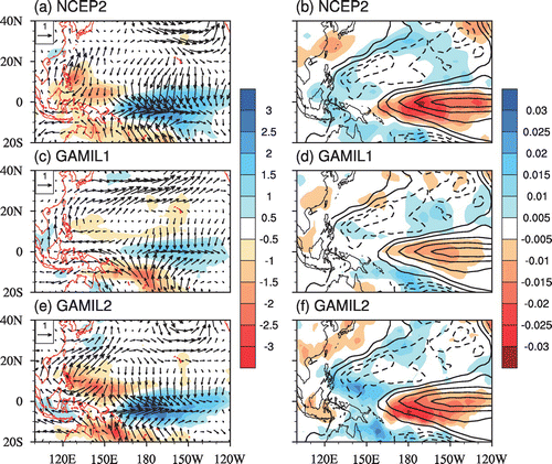
Figure 3. Regression coefficients of the December–January–February 1000-hPa winds (vectors; m s−1), precipitation (left column; shaded; mm d−1), 500-hPa omega (right column; shaded; pa s−1), and SST (contours; °C) with respect to the Niño3.4 index derived from (a, b) the observation (NCEP-2), (c, d) GAMIL1, and (e, f) GAMIL2.

Figure 4. Regression coefficients of the December–January–February heating rate (K d−1) vertically integrated from 1000 to 200 hPa in total moist processes with respect to the Niño3.4 index derived from (a) the observation (CFSR), (b) GAMIL1, (c) GAMIL2, and (d) the difference between GAMIL2 and GAMIL1.
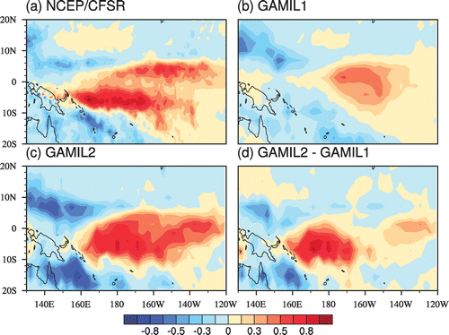
Figure 4. Regression coefficients of the December–January–February heating rate (K d−1) vertically integrated from 1000 to 200 hPa in total moist processes with respect to the Niño3.4 index derived from (a) the observation (CFSR), (b) GAMIL1, (c) GAMIL2, and (d) the difference between GAMIL2 and GAMIL1.