Combined impact of the Pacific–Japan pattern and Mediterranean–northern Eurasia pattern on East Asian summer temperatures

Figures & data

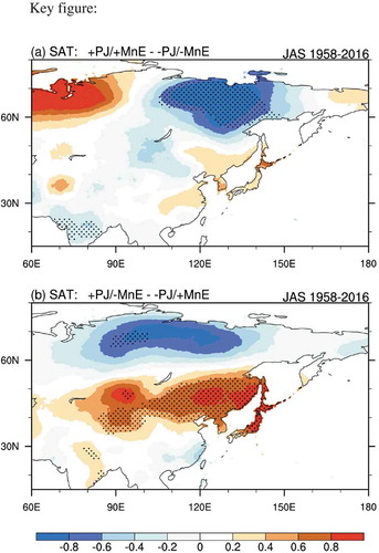
Figure 1. Normalized time series of the PJ and MnE indices during summer over the period 1958–2016. Solid lines indicate the +0.5/−0.5 standard deviations.

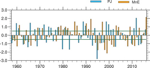
Figure 2. Regressed geopotential height (shading; units: gpm) and wind (vectors; units: m s⁻¹) anomalies at (a) 850 hPa, (b) 500 hPa, and (c) 200 hPa against the PJ index during summer over the period 1958–2016. (d–f) As in (a–c) but against the MnE index. The dotted areas are geopotential height anomalies significant at the 95% confidence level. Arrows are the wind anomalies significant at the 95% confidence level. The green box in Figure 2(d) represents the domain used to define the MnE index.

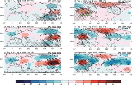
Figure 3. Regression maps of the total radiation flux (units: W m⁻²) against the (a) PJ and (b) MnE indices during summer over the period 1958–2016. (c, d) As in (a, b) but for the SAT (units: °C). The dotted areas are significant at the 95% confidence level.

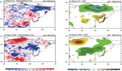
Table 1. List of +PJ/+MnE, +PJ/−MnE, −PJ/+MnE, and −PJ/−MnE years over the period 1958–2016.

	+PJ	−PJ
+MnE	1961 1978 1981 1982 1990 2004 2016	1964 1969 1971 1980 1992 1997 2003 2013
−MnE	1960 1966 1968 1977 1994 1999 2000 2001 2002 2011	1958 1963 1965 1995 1998 2010 2014

Figure 4. Composite differences in the geopotential height (units: gpm) and wind (vectors; units: m s⁻¹) at (a) 850 hPa, (b) 500 hPa, and (c) 200 hPa between the +PJ/+MnE and −PJ/−MnE years during summer over the period 1958–2016. (d–f) As in (a–c) but between the +PJ/−MnE and +PJ/−MnE years. The dotted areas are geopotential height anomalies significant at the 95% confidence level. Arrows are the wind anomalies significant at the 95% confidence level.

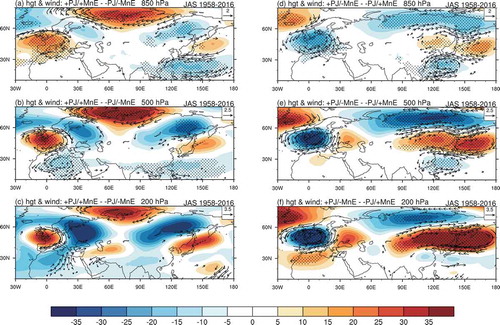
Figure 5. Composite differences in the SAT (units: °C) (a) between the +PJ/+MnE and −PJ/−MnE years and (b) between the +PJ/−MnE and −PJ/+MnE years during summer over the period 1958–2016. The dotted areas are significant at the 95% confidence level.

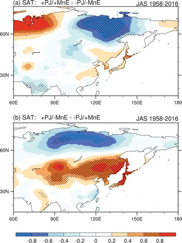
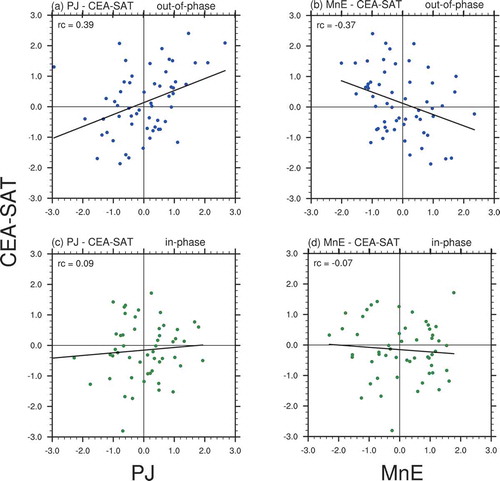
Figure 6. Scatterplots of the CEA-SAT versus the (a) PJ and (b) MnE indices during summer over the period 1958–2016. (c, d) as in (a, b) but for out-of-phase PJ-MnE years, respectively. (e, f) as in (a, b) but for in-phase PJ-MnE years, respectively.

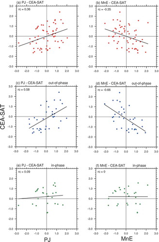
Figure 7. Scatterplots of the CEA-SAT versus the (a) PJ and (b) MnE indices during summers in out-of-phase PJ-MnE years over the period 1901–2010 using ERA-20C SLP and CRU SAT data. (c, d) as in (a, b) but for in-phase PJ-MnE years, respectively.